![]()
Update 28 Feb 2019: I added a new blog post with a slide deck containing the presentation I did for PyData Montreal.
Today, at the PyTorch Developer Conference, the PyTorch team announced the plans and the release of the PyTorch 1.0 preview with many nice features such as a JIT for model graphs (with and without tracing) as well as the LibTorch, the PyTorch C++ API, one of the most important release announcement made today in my opinion.
Given the huge interest in understanding how this new API works, I decided to write this article showing an example of many opportunities that are now open after the release of the PyTorch C++ API. In this post, I’ll integrate PyTorch inference into native NodeJS using NodeJS C++ add-ons, just as an example of integration between different frameworks/languages that are now possible using the C++ API.
Below you can see the final result:
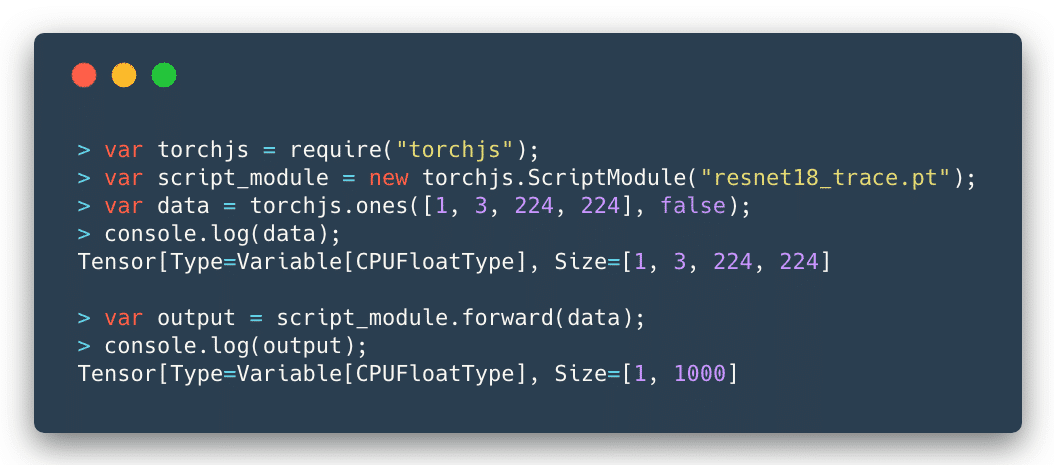
As you can see, the integration is seamless and I could use a traced ResNet as the computational graph model and feed any tensor to it to get the output predictions.
Introduction
Simply put, the libtorch is a library version of the PyTorch. It contains the underlying foundation that is used by PyTorch, such as the ATen (the tensor library), which contains all the tensor operations and methods. Libtorch also contains the autograd, which is the component that adds the automatic differentiation to the ATen tensors.
A word of caution for those who are starting now is to be careful with the use of the tensors that can be created both from ATen and autograd, do not mix them, the ATen will return the plain tensors (when you create them using the at namespace) while the autograd functions (from the torch namespace) will return Variable, by adding its automatic differentiation mechanism.
For a more extensive tutorial on how PyTorch internals work, please take a look on my previous tutorial on the PyTorch internal architecture.
Libtorch can be downloaded from the Pytorch website and it is only available as a preview for a while. You can also find the documentation in this site, which is mostly a Doxygen rendered documentation. I found the library pretty stable, and it makes sense because it is actually exposing the stable foundations of PyTorch, however, there are some issues with headers and some minor problems concerning the library organization that you might find while starting working with it (that will hopefully be fixed soon).

For NodeJS, I’ll use the Native Abstractions library (nan) which is the most recommended library (actually is basically a header-only library) to create NodeJS C++ add-ons and the cmake-js, because libtorch already provide the cmake files that make our building process much easier. However, the focus here will be on the C++ code and not on the building process.
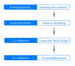
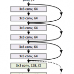
The flow for the development, tracing, serializing and loading the model can be seen in the figure on the left side.
It starts with the development process and tracing being done in PyTorch (Python domain) and then the loading and inference on the C++ domain (in our case in NodeJS add-on).
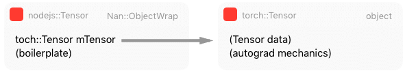
Wrapping the Tensor
In NodeJS, to create an object as a first-class citizen of the JavaScript world, you need to inherit from the ObjectWrap class, which will be responsible for wrapping a C++ component.
#ifndef TENSOR_H
#define TENSOR_H

#include <nan.h>
#include <torch/torch.h>

namespace torchjs {

class Tensor : public Nan::ObjectWrap {
 public:
  static NAN_MODULE_INIT(Init);

  void setTensor(at::Tensor tensor) {
    this->mTensor = tensor;
  }

  torch::Tensor getTensor() {
    return this->mTensor;
  }

  static v8::Local<v8::Object> NewInstance();

 private:
  explicit Tensor();
  ~Tensor();

  static NAN_METHOD(New);
  static NAN_METHOD(toString);
  static Nan::Persistent<v8::Function> constructor;

 private:
  torch::Tensor mTensor;

};

}  // namespace torchjs

#endif
As you can see, most of the code for the definition of our Tensor class is just boilerplate. The key point here is that the torchjs::Tensor will wrap a torch::Tensor and we added two special public methods (setTensor and getTensor) to set and get this internal torch tensor.
I won’t show all the implementation details because most parts of it are NodeJS boilerplate code to construct the object, etc. I’ll focus on the parts that touch the libtorch API, like in the code below where we are creating a small textual representation of the tensor to show on JavaScript (toString method):
NAN_METHOD(Tensor::toString) {
  Tensor* obj = ObjectWrap::Unwrap<Tensor>(info.Holder());
  std::stringstream ss;

  at::IntList sizes = obj->mTensor.sizes();
  ss << "Tensor[Type=" << obj->mTensor.type() << ", ";
  ss << "Size=" << sizes << std::endl;

  info.GetReturnValue().Set(Nan::New(ss.str()).ToLocalChecked());
}
What we are doing in the code above, is just getting the internal tensor object from the wrapped object by unwrapping it. After that, we build a string representation with the tensor size (each dimension sizes) and its type (float, etc).
Wrapping Tensor-creation operations
Let’s create now a wrapper code for the torch::ones function which is responsible for creating a tensor of any defined shape filled with constant 1’s.
NAN_METHOD(ones) {
  // Sanity checking of the arguments
  if (info.Length() < 2)
    return Nan::ThrowError(Nan::New("Wrong number of arguments").ToLocalChecked());

  if (!info[0]->IsArray() || !info[1]->IsBoolean())
    return Nan::ThrowError(Nan::New("Wrong argument types").ToLocalChecked());

  // Retrieving parameters (require_grad and tensor shape)
  const bool require_grad = info[1]->BooleanValue();
  const v8::Local<v8::Array> array = info[0].As<v8::Array>();
  const uint32_t length = array->Length();

  // Convert from v8::Array to std::vector
  std::vector<long long> dims;
  for(int i=0; i<length; i++)
  {
    v8::Local<v8::Value> v;
    int d = array->Get(i)->NumberValue();
    dims.push_back(d);
  }

  // Call the libtorch and create a new torchjs::Tensor object
  // wrapping the new torch::Tensor that was created by torch::ones
  at::Tensor v = torch::ones(dims, torch::requires_grad(require_grad));
  auto newinst = Tensor::NewInstance();
  Tensor* obj = Nan::ObjectWrap::Unwrap<Tensor>(newinst);
  obj->setTensor(v);

  info.GetReturnValue().Set(newinst);
}
So, let’s go through this code. We are first checking the arguments of the function. For this function, we’re expecting a tuple (a JavaScript array) for the tensor shape and a boolean indicating if we want to compute gradients or not for this tensor node. After that, we’re converting the parameters from the V8 JavaScript types into native C++ types. Soon as we have the required parameters, we then call the torch::ones function from the libtorch, this function will create a new tensor where we use a torchjs::Tensor class that we created earlier to wrap it.
And that’s it, we just exposed one torch operation that can be used as native JavaScript operation.
Intermezzo for the PyTorch JIT
The introduced PyTorch JIT revolves around the concept of the Torch Script. A Torch Script is a restricted subset of the Python language and comes with its own compiler and transform passes (optimizations, etc).
This script can be created in two different ways: by using a tracing JIT or by providing the script itself. In the tracing mode, your computational graph nodes will be visited and operations recorded to produce the final script, while the scripting is the mode where you provide this description of your model taking into account the restrictions of the Torch Script.
Note that if you have branching decisions on your code that depends on external factors or data, tracing won’t work as you expect because it will record that particular execution of the graph, hence the alternative option to provide the script. However, in most of the cases, the tracing is what we need.
To understand the differences, let’s take a look at the Intermediate Representation (IR) from the script module generated both by tracing and by scripting.
@torch.jit.script
def happy_function_script(x):
    ret = torch.rand(0)
    if True == True:
        ret = torch.rand(1)
    else:
        ret = torch.rand(2)
    return ret

def happy_function_trace(x):
    ret = torch.rand(0)
    if True == True:
        ret = torch.rand(1)
    else:
        ret = torch.rand(2)
    return ret

traced_fn = torch.jit.trace(happy_function_trace,
                            (torch.tensor(0),),
                            check_trace=False)
In the code above, we’re providing two functions, one is using the @torch.jit.script decorator, and it is the scripting way to create a Torch Script, while the second function is being used by the tracing function torch.jit.trace. Not that I intentionally added a “True == True” decision on the functions (which will always be true).
Now, if we inspect the IR generated by these two different approaches, we’ll clearly see the difference between the tracing and scripting approaches:
# 1) Graph from the scripting approach
graph(%x : Dynamic) {
%16 : int = prim::Constant[value=2]()
%10 : int = prim::Constant[value=1]()
%7 : int = prim::Constant[value=1]()
%8 : int = prim::Constant[value=1]()
%9 : int = aten::eq(%7, %8)
%ret : Dynamic = prim::If(%9)
block0() {
%11 : int[] = prim::ListConstruct(%10)
%12 : int = prim::Constant[value=6]()
%13 : int = prim::Constant[value=0]()
%14 : int[] = prim::Constant[value=[0, -1]]()
%ret.2 : Dynamic = aten::rand(%11, %12, %13, %14)
-> (%ret.2)
}
block1() {
%17 : int[] = prim::ListConstruct(%16)
%18 : int = prim::Constant[value=6]()
%19 : int = prim::Constant[value=0]()
%20 : int[] = prim::Constant[value=[0, -1]]()
%ret.3 : Dynamic = aten::rand(%17, %18, %19, %20)
-> (%ret.3)
}
return (%ret);
}
# 2) Graph from the tracing approach
graph(%0 : Long()) {
%7 : int = prim::Constant[value=1]()
%8 : int[] = prim::ListConstruct(%7)
%9 : int = prim::Constant[value=6]()
%10 : int = prim::Constant[value=0]()
%11 : int[] = prim::Constant[value=[0, -1]]()
%12 : Float(1) = aten::rand(%8, %9, %10, %11)
return (%12);
}
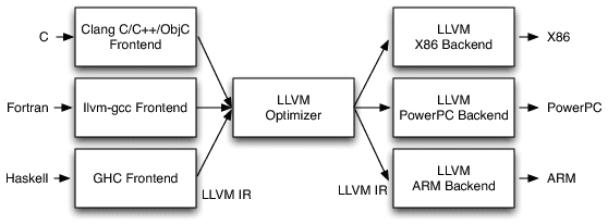
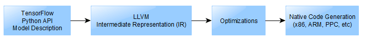
As we can see, the IR is very similar to the LLVM IR, note that in the tracing approach, the trace recorded contains only one path from the code, the truth path, while in the scripting we have both branching alternatives. However, even in scripting, the always false branch can be optimized and removed with a dead code elimination transform pass.
PyTorch JIT has a lot of transformation passes that are used to do loop unrolling, dead code elimination, etc. You can find these passes here. Not that conversion to other formats such as ONNX can be implemented as a pass on top of this intermediate representation (IR), which is quite convenient.
Tracing the ResNet
Now, before implementing the Script Module in NodeJS, let’s first trace a ResNet network using PyTorch (using just Python):
traced_net = torch.jit.trace(torchvision.models.resnet18(),
                             torch.rand(1, 3, 224, 224))
traced_net.save("resnet18_trace.pt")
As you can see from the code above, we just have to provide a tensor example (in this case a batch of a single image with 3 channels and size 224×224. After that we just save the traced network into a file called resnet18_trace.pt.
Now we’re ready to implement the Script Module in NodeJS in order to load this file that was traced.
Wrapping the Script Module
This is now the implementation of the Script Module in NodeJS:
// Class constructor
ScriptModule::ScriptModule(const std::string filename) {
  // Load the traced network from the file
  this->mModule = torch::jit::load(filename);
}

// JavaScript object creation
NAN_METHOD(ScriptModule::New) {
  if (info.IsConstructCall()) {
    // Get the filename parameter
    v8::String::Utf8Value param_filename(info[0]->ToString());
    const std::string filename = std::string(*param_filename);

    // Create a new script module using that file name
    ScriptModule *obj = new ScriptModule(filename);
    obj->Wrap(info.This());
    info.GetReturnValue().Set(info.This());
  } else {
    v8::Local<v8::Function> cons = Nan::New(constructor);
    info.GetReturnValue().Set(Nan::NewInstance(cons).ToLocalChecked());
  }
}
As you can see from the code above, we’re just creating a class that will call the torch::jit::load function passing a file name of the traced network. We also have the implementation of the JavaScript object, where we convert parameters to C++ types and then create a new instance of the torchjs::ScriptModule.
The wrapping of the forward pass is also quite straightforward:
NAN_METHOD(ScriptModule::forward) {
  ScriptModule* script_module = ObjectWrap::Unwrap<ScriptModule>(info.Holder());
  Nan::MaybeLocal<v8::Object> maybe = Nan::To<v8::Object>(info[0]);

  Tensor *tensor =
    Nan::ObjectWrap::Unwrap<Tensor>(maybe.ToLocalChecked());

  torch::Tensor torch_tensor = tensor->getTensor();
  torch::Tensor output = script_module->mModule->forward({torch_tensor}).toTensor();

  auto newinst = Tensor::NewInstance();
  Tensor* obj = Nan::ObjectWrap::Unwrap<Tensor>(newinst);
  obj->setTensor(output);
  info.GetReturnValue().Set(newinst);
}
As you can see, in this code, we just receive a tensor as an argument, we get the internal torch::Tensor from it and then call the forward method from the script module, we wrap the output on a new torchjs::Tensor and then return it.
And that’s it, we’re ready to use our built module in native NodeJS as in the example below:
var torchjs = require("./build/Release/torchjs");
var script_module = new torchjs.ScriptModule("resnet18_trace.pt");
var data = torchjs.ones([1, 3, 224, 224], false);
var output = script_module.forward(data);
I hope you enjoyed ! Libtorch opens the door for the tight integration of PyTorch in many different languages and frameworks, which is quite exciting and a huge step towards the direction of production deployment code.
– Christian S. Perone
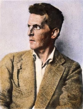 One of the most interesting aspects of Wittgenstein is perhaps that fact that he had developed two very different philosophies during his life, and each of which had great influence. Something quite rare for someone who spent so much time working on these ideas and retreating even after the major influence they exerted, especially in the Vienna Circle. A true lesson of intellectual honesty, and in my opinion, one important legacy.
 John R. Firth
")
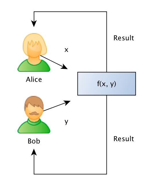
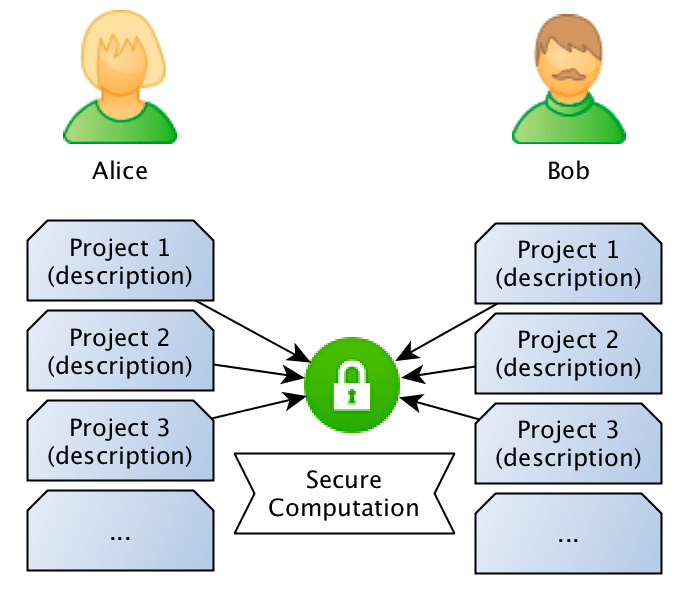 What they want to do is to jointly compute the similarity between projects in order to find if they should be doing partnership on a project or not, however, and this is the important point: Bob doesn’t want Alice to know the project descriptions and neither Alice wants Bob to be aware of their projects, they want to know the closest match between the different projects they run, but without disclosing the project ideas (project descriptions).
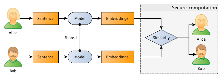
 = \frac {\pmb x \cdot \pmb y}{||\pmb x|| \cdot ||\pmb y||}")
 =\hat{x} \cdot\hat{y}")

-5)+100)") , where I intentionally added redundant operations to see LLVM constant propagation later.
, where I intentionally added redundant operations to see LLVM constant propagation later.