Note: This is a continuation of the previous post: Thoughts on Riemannian metrics and its connection with diffusion/score matching [Part I], so if you haven’t read it yet, please consider reading as I won’t be re-introducing in depth the concepts (e.g., the two scores) that I described there already. This article became a bit long, so if you are familiar already with metric tensors and differential geometry you can just skip the first part.

I was planning to write a paper about this topic, but my spare time is not that great so I decided it would be much more fun and educative to write this article in form of a tutorial. If you liked it, please consider citing it:

Introduction

I’m writing this second part of the series because I couldn’t find any formalisation of this metric tensor that naturally arises from the Stein score (especially when used with learned models), and much less blog posts or articles about it, which is surprising given its deep connection between score-based generative models, diffusion models and the geometry of the data manifold. I think there is an emerging field of “data geometry” that will be as impactful as information geometry (where the Stein score “counterpart”, the Fisher information, is used to construct the Fisher information metric tensor, the statistical manifold metric tensor – a fun fact, I used to live very close to where Fisher lived his childhood in north London). It is very unfortunate though, that the term “Geometric Deep Learning” has become a synonymous of Deep Learning on graphs when there is so much more about it to be explored.

As you will see later, this metric tensor opens up new possibilities for defining data-driven geometries that adapt to the data manifold. One thing that became clear to me is that score-based generative models tells data how to move and data tells score-based generative models how to curve, and given the connection of score-based models and diffusion, this is a very exciting area to explore and where we can find many interesting connections and the possibility to use the entire framework of differential geometry, which is a quite unique perspective in how we see these models and what they are learning.

I have made many simplifications to make this an educative article instead of just dumping formulas and definitions, the motivation is mainly because differential geometry and tensor calculus is usually not very common in ML outside of the information geometry domain, geometric deep learning and physics. The examples I will show below using a 2D gaussian distribution are one example – it is obviously easier to find geodesics without relying on optimisation, but I’m assuming this could be a much more complex model of score estimation and thus consider it a black-box instead of considering the analytical definition of a gaussian and carry on with simplifications.

Manifolds \(M\) and Tangent Spaces \(T_pM\)

If you work in ML, you probably heard about the manifold hypothesis already, this hypothesis posits that “many high-dimensional data sets that occur in the real world actually lie along low-dimensional latent manifolds inside that high-dimensional space“. This doesn’t tell you, however, what a manifold actually is, especially the intuition, so I will give a basic intuition and define it while trying to focus on the tangent space, which is essential to understand the metric tensor that I will talk about it later. I won’t go through all components of a manifold and will try to keep it high level with a focus on what we need to understand the metric tensor.

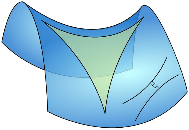
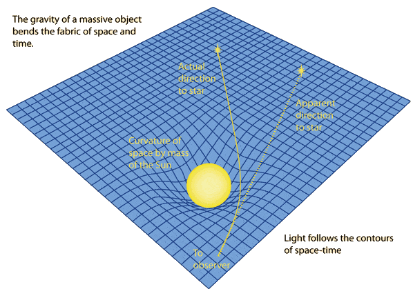
So, imagine stretching and bending a piece of rubber without tearing (or gluing it :D). The resulting shape, no matter how complex, captures the essence of a smooth manifold. These manifolds are surfaces or higher-dimensional spaces that locally resemble flat Euclidean space, but globally can take on rich structure, just like the structure of our universe (e.g., see the image at the top of the post showing gravitational lensing). Now, formally, a smooth manifold is a topological space that is locally homeomorphic to Euclidean space and has a smooth structure. This means that around each point, we can find a neighbourhood that looks just like a piece of \(\mathbb{R}^n\), and the transitions between these local views are smooth.

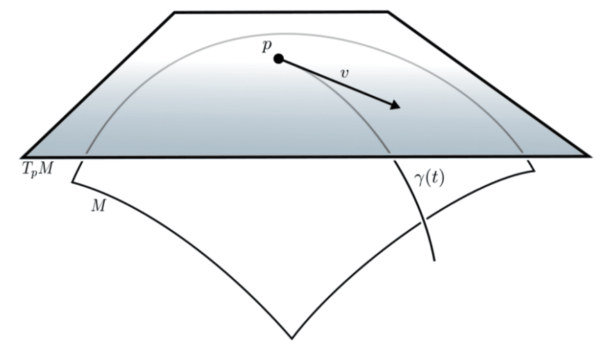
Now, at each point \(p\) on a manifold, we can imagine all possible directions in which we could move. These directions form a vector space called the tangent space, which serves as a local linear approximation of the manifold at that point. The notation used for it is usually \(T_pM\), which means the tangent space \(T\) of the manifold \(M\) at the point \(p\). You can see in the image on the left the point \(p\) in the manifold and the cross section there showing the tangent space \(T_pM\). You can also see a curve \(\gamma(t)\) representing a geodesic, but I will talk about the geodesics a bit later once we have the metric tensor. Later on we will be using stochastic gradient descent (SGD) to optimize a discrete “curve” path made of multiple segments using the metric tensor we will define.
While the tangent space provides a linear approximation of the manifold at a point, it still doesn’t allow us to be able to define lengths, vectors or angles between them (we still cannot calculate an inner product), for this we will need the metric tensor, which we will talk about it below.

Metric tensor \(g\): equipping the inner product \(\langle u, v \rangle\)

Imagine you’re an ant walking on the surface of an orange. To you, and to flat earthers especially (although ants have the license to believe in it), the world seems flat, yet you’re traversing a curved surface in a higher-dimensional space. At the very core of differential geometry, we have the metric tensor, which we call a tensor but it is actually a tensor field.
There is often a confusion between the metric tensor in differential geometry and the one in metric spaces or measure theory (here we are again in the overloading issues, which can get much worse if you start using tensor calculus notation with lower and upper indicies). In a metric space, a metric refers to a function that defines the distance between two points (e.g., the Euclidean distance).
Now, the metric tensor is a different animal, it is a tensor field on a manifold that defines an inner product \(\langle \cdot, \cdot \rangle\) on the tangent space at each point, so that we can use it to compute distances and angles (locally, by integrating along curves). It is basically a generalisation of the idea of distance on curved spaces (as opposed to flat spaces), but we will get concrete with this later and it will be clear when you actually see the code, especially if you never used a metric tensor before (although you have been using one all the time, the identity metric tensor, which is the metric tensor that induces the dot product in Euclidean geometry).

The metric tensor is often denoted by \(g\) symbol and it is defined as:

$$ g_p: T_pM \times T_pM \rightarrow \mathbb{R}, p \in M $$

Where we have the \(g_p\) which is the metric tensor at the point \(p\). You can also find the notation as \(g_x\) which is at the point \(x\), as I will use later because this will become data samples and we often denote data with \(x\) in ML. We also have the tangent space \(T_pM\) and manifold \(M\) that we mentioned before and the \(T_pM \times T_pM \rightarrow \mathbb{R}\) which tells us that the metric tensor takes two vectors from the tangent space as input and maps to the real numbers. The most important thing you need to understand here is that the \(g_p\) can be different for each point \(p\) (or constant everywhere as in Euclidean flat spaces). I think a good intuition to understand the metric tensor is to think that at every point in a curved space you have a curvature and this curvature can change depending on where you are in this curved space, therefore you need a “measuring stick” to be able to compute inner products, without that you cannot compute lengths because you don’t know how much each axis will stretch or contract. We will see that our new tensor derived from the Stein score will change at every point in space according to the learned data curvature, which is very interesting in my opinion.

One interesting parallel we can take here is the Fisher information metric (not to be confused with the Fisher information) where each point \(p\) is actually a different parametrisation of a distribution in the statistical manifold. You can see a very nice animation tool that shows you a geodesic (we will talk about what this means soon) between two gaussian distributions that can have different parametrisation, so you can compute a distance between distributions in the statistical manifold using the Fisher information metric. This metric tensor is basically the core of information geometry, which is dealing with distribution parameters as the point \(p\), allowing you to compute inner products, distances, lengths, geodesics, angles in the statistical manifold. For more information about it and the relationship of the Fisher information metric with optimization and its use in natural gradient please take a look at my slides about gradient-based optimization.

Now, I made this parallel because the form of the Fisher information is very similar to what we will do, except that in our metric tensor constructed from the Stein score we will define each point \(p\) not as parameters of a distribution but as the data itself. The Fisher metric tensor will tell you the curvature in the statistical manifold, of the information geometry, and our metric tensor built from the Stein score will tell us the curvature of the data geometry.

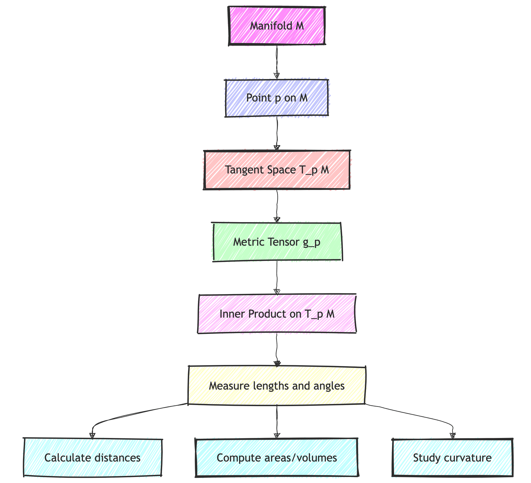
Here is where we stand now in terms of concepts that we learned:

Example: Metric tensor \(g\) in Euclidean space

The simplest metric tensor we can use as an example is the metric tensor in the Euclidean space \(\mathbb{R}^n\), in this case it is defined as:

$$ g = I_n $$

Where \(I_n\) is the \(n \times n\) identity matrix for \(\mathbb{R}^n\). Now, let’s use this metric tensor to compute the inner product and see where we end up. To compute the inner product, we just do:

$$ \langle u, v \rangle_g = u^T g v $$

Note that we are omitting here the point because this metric tensor is the same everywhere (it is constant everywhere), but one could write the inner product definition as \( \langle u, v \rangle_g(x)\) where \(x\) is the point where the metric tensor is evaluated at (which can be different than \(u\) and \(v\) as we will see later in an example). So let’s plug now our metric tensor definition, which is the identity matrix, and therefore we will have an enormous simplification:

$$ \langle u, v \rangle_g = u^T I_n v = u^T v $$

The inner product is simply the dot product of the vectors \(u\) and \(v\), which we are very familiar with. The identity matrix does not change the computation, but it’s important to understand that the metric tensor in this case is \(I_n\).

Note that the inner product immediately induces a norm as well:

$$ \|v\|_g = \sqrt{\langle v, v \rangle_g} $$

Thus, the norm \(\|v\|_g\) represents the length of the vector \(v\) in the geometry defined by the metric tensor \(g\).

While in Euclidean space the metric tensor is the identity matrix and simply gives us the standard dot product, it becomes more interesting on curved or more complex manifolds. In these cases, the metric tensor varies from point to point and encodes the curvature and structure of the space. Distances and angles in such spaces are no longer as simple as in the Euclidean case, but the same principles apply: the metric tensor provides the framework for computing inner products, distances, and angles, adapted to the specific geometry of the manifold.

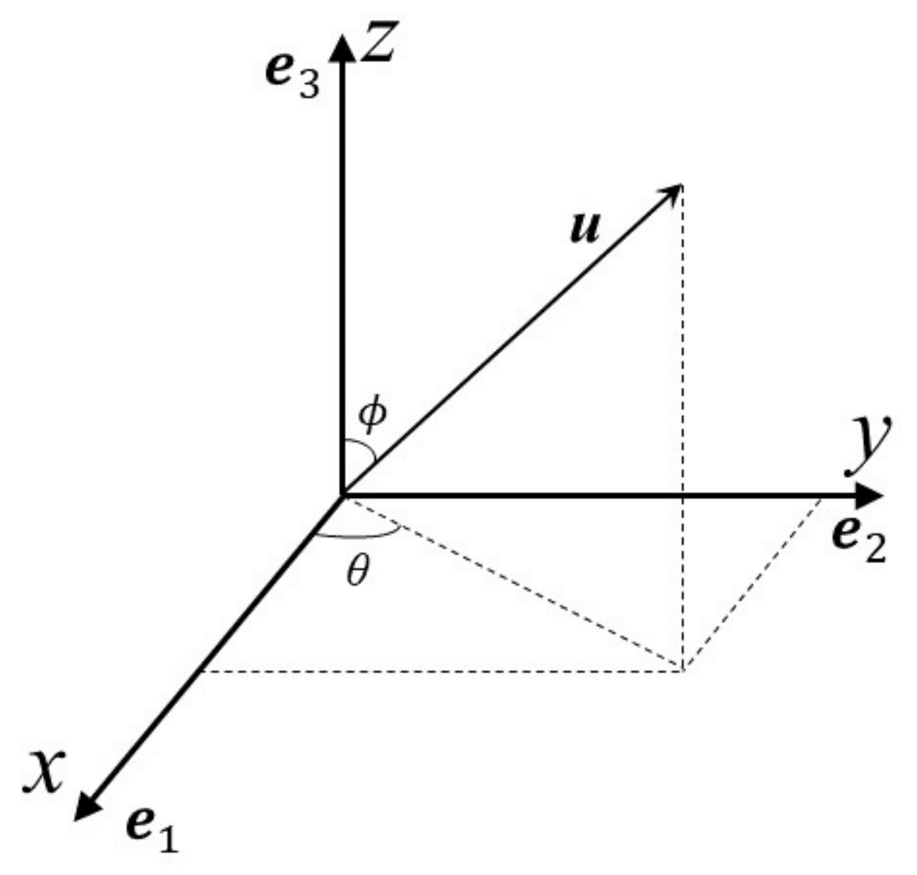
Now, if you want to understand a bit better how the identity matrix suddenly appears as the metric tensor for the Euclidean space, you need to understand basis vectors. They basically (or basically ? I know I should stop with these bad jokes) provide a set of directions that we use to describe any vector in a space. In 3D space (\(\mathbb{R}^3\)) for example, the standard basis vectors point along the x, y, and z axes and any vector can be represented as a combination of these basis vectors, using a certain amount of each, we just combine them. In the end, the intuitive view that you can have is that they act like a coordinate system, that allows us to describe and navigate that space.

The standard basis vectors for a 3D space are the following:

$$\mathbf{e}_1 = \begin{pmatrix} 1 \\ 0 \\ 0 \end{pmatrix}, \quad
\mathbf{e}_2 = \begin{pmatrix} 0 \\ 1 \\ 0 \end{pmatrix}, \quad
\mathbf{e}_3 = \begin{pmatrix} 0 \\ 0 \\ 1 \end{pmatrix}$$

Each one is pointing to a direction, now you get where the Euclidean metric tensor (the identity matrix) comes from:

$$ g_{ij} = \delta_{ij} = \begin{pmatrix} 1 & 0 & 0 \\ 0 & 1 & 0 \\ 0 & 0 & 1 \end{pmatrix} $$

Where \(\delta_{ij}\) is the Kronecker Delta, that gives is the simple rule below that makes it convenient to represent the Euclidean orthonormal metric tensor:

$$ \delta_{ij} =
\begin{cases}
1 & \text{if } i = j \\
0 & \text{if } i \neq j
\end{cases} $$

One misconception that is often very common is to think that the Euclidean space is not a Riemannian manifold, but it actually is. A Riemannian manifold is basically a manifold that has more structure, such as a smoothly varying and positive definite metric tensor. The identity matrix used in Euclidean space meets this criteria, so the Euclidean manifold is indeed a Riemannian manifold when equipped with its standard positive-definite metric tensor (the identity matrix).

That’s enough for our Euclidean example, let’s jump now on how we define curves and geodesics on a manifold.

Curves \(\gamma(t)\) and Geodesics

Curves, Length and Energy

Let’s shift now the focus to curves first. A curve on a manifold is a smooth path \(\gamma(t)\) parameterized by \(t\) that traces a path between two points on the manifold. The natural way to measure the length of a curve is by integrating the infinitesimal distances along the curve, however, now that we know that a metric tensor \(g\) exists, we will integrate these infinitesimal distances using the inner product equipped with the metric tensor:

$$ L[\gamma] = \int_0^1 \sqrt{\underbrace{\langle \dot{\gamma}(t), \dot{\gamma}(t) \rangle_g}_{\text{Inner product}}} \, dt $$

The 0 to 1 integration you see in the equation means that 0 is the beginning of the curve and 1 is the end of it (as parametrized by \(t \in \left[0, 1\right]\)). This curve maps from the interval \(\left[0, 1\right]\) into a manifold \(M\), i.e., \(\gamma(t) : \left[0, 1\right] \rightarrow M\). At each value of \(t\), \(\gamma(t)\) gives a point on the manifold. You might not be used to the dot at top of the \(\dot{\gamma}\) curve, as it is not common in ML to use that notation, but this notation basically means that we are taking the derivative of the curve with respect to the parameter \(t\):

$$ \dot{\gamma}(t) = \frac{d}{dt}\gamma(t) $$

Understanding the length formula is very simple, the squared root of the \(\langle \dot{\gamma}(t), \dot{\gamma}(t) \rangle_g\) gives the instantaneous speed at each point along the curve and the integral is accumulating the “instantaneous distances” as you move along the curve from \(t=0\) to \(t=1\). This accumulation gives the total distance traveled, or the length of the curve, and given that we are using the metric tensor \(g\), it will give us the length of the curve on the manifold, taking into consideration the local curvature along the way.

One important definition here that might help understand a bit better as well, is that the \(L[\gamma]\) is a functional, which is a special type of mathematical object that maps functions to real numbers. More specifically, it’s a function that takes another function (or curve) as its input and outputs a scalar.

You now probably have a good idea of what the length is computing and how we built the understanding coming from the inner product definition equipped with the metric tensor. Let’s now talk about an even simpler concept which is the energy functional \(E[\gamma]\) defined below:

$$ E[\gamma] = \int_0^1 \langle \dot{\gamma}(t), \dot{\gamma}(t) \rangle_g \, dt $$

This is very similar to the length, except that we don’t have the square root. The reason why energy is more convenient, and we will see later a concrete example when we start optimizing geodesics using energy, is that since energy depends quadratically on the velocity, it has better analytic properties (e.g. smoothness). Note bracket in the notation to denote that it is a functional (it is taking the \(\gamma\) curve that is used for the integration).

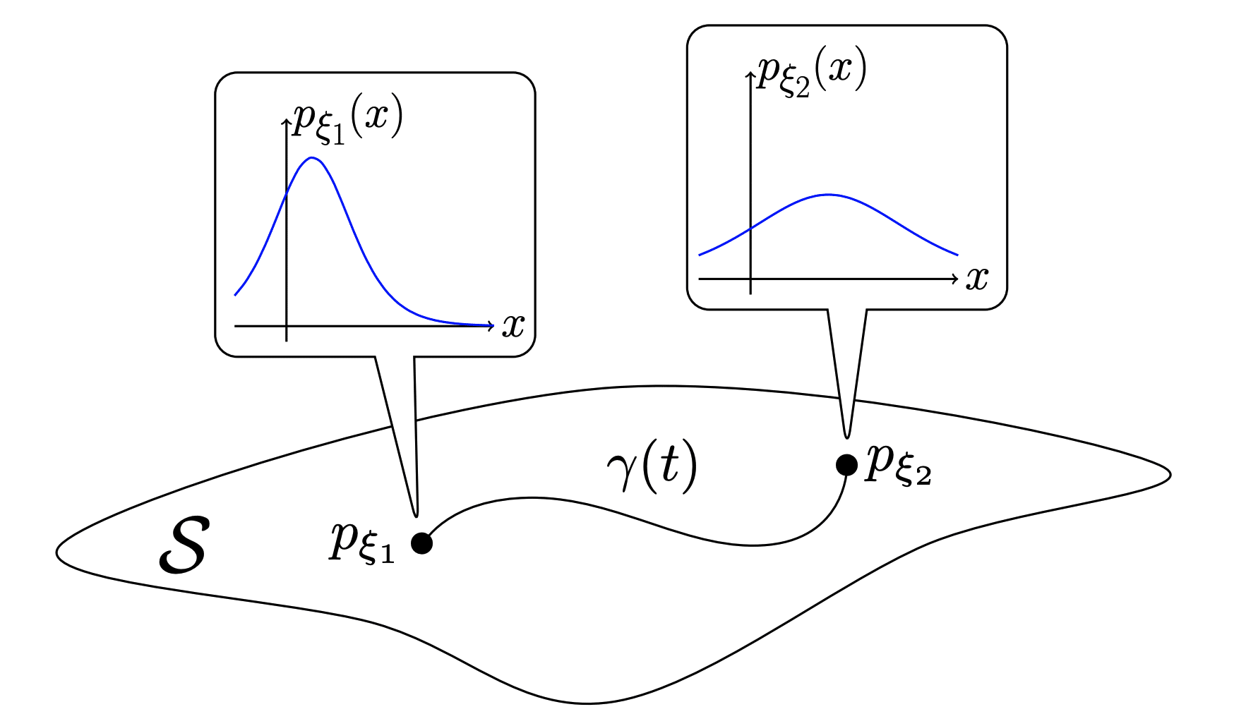
Let’s think now in an interesting example from information geometry. Remember that we mentioned that in information geometry you are dealing with the statistical manifold ? We can define curves in this statistical manifold where each point \(p\) actually represents the parameters of a distribution. A very simple example is a gaussian distribution, you can think that each point in the statistical manifold represents a valid parametrisation of the gaussian distribution. In the figure in the left, we can see the two points and their respective gaussians. Note as well that we can make curves between these distributions such as the \(\gamma(t)\) shown in the figure connecting the two gaussians.

In Euclidean spaces, a shortest path is always a straight path between points. But on more complex and rich manifolds, this concept doesn’t apply anymore. The way we find the shortest path between points is by finding this curve that minimizes the length between points, which we call a “geodesic”, although a geodesic might not always globally be the shortest path and we will see later the limitations of minimizing the energy to find a geodesic between points.

 

Geodesics

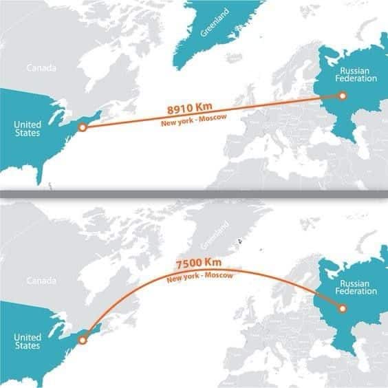
Geodesics are a special kind of curve that represent the shortest path (again, not always globally) between two points on the manifold, much like a straight line in Euclidean space. Geodesics are defined by the metric tensor that we just introduced, and they are crucial for understanding the intrinsic geometry of the manifold.
Now, in data geometry, geodesics reflect the natural paths between data points, with distances defined by the data manifold itself. This helps us understand the “shape” of the data and explore relationships between points in a geometrically meaningful way. Note the difference here between the data manifold where the points represent data samples and the statistical manifold from information geometry where points represent parametrisations of a distribution. We will focus here in the data manifold, where we will use later the Stein score to build a metric tensor for this manifold.

The easiest way to understand geodesics is by imagining that you want to get from point A to point B using the least possible effort (or Energy, as we just talked in the previous sections), you’ll naturally follow what’s called a “great circle” – like how airplanes follow curved paths on long-distance flights that look strange on flat maps but are actually shortest paths. In differential geometry, a geodesic generalizes this idea to any curved surface or space. It’s the path that an object would follow if it were moving “straight ahead” without any external forces – just following the natural curvature of the space it’s in.

Geodesics as energy minimization

You can solve geodesic equations (that use Christoffel symbols) using many different methods. I will focus here, however, into how we can find a geodesic through an optimization perspective (because we are a ML community and we love optimization). My focus here is not to provide you an extensive collection of methods on how you can find geodesics, my focus is to give you the understanding of the geodesics that will show up later and the tools needed to find it. There are obviously many things you can do when you are dealing with very simple expressions, but when we take learned networks into the equation, things become much more expensive and difficult, for that reason I’m trying to provide a way to find geodesics assuming that the Stein score that we will be using later is a black box (e.g. was learned with a deep neural network), hence why the optimization perspective is a good fit here.

Let’s review the Energy functional that we introduced earlier:

$$ E[\gamma] = \int_0^1 \langle \dot{\gamma}(t), \dot{\gamma}(t) \rangle_g \, dt $$

All critical points of the energy functional correspond to geodesics, but these critical points can be of different types (minima, maxima, or saddle points), for our problem we won’t have issues with saddle points but it is good to know (if you are interested in learning more about it, Keenan has an amazing video on it, with the most beautiful slide deck you will ever find in differential geometry).

The goal of our optimization will be to find the curve \(\gamma\) that minimizes this energy functional \(E[\gamma]\), this would be:

$$ \theta^\ast = \arg \min_{\theta} E[\gamma_\theta] = \arg \min_{\theta} \left( \frac{1}{2} \int_{a}^{b} \langle \dot{\gamma}(t; \theta), \dot{\gamma}(t; \theta) \rangle_g \, dt \right) $$

where the \(\theta\) are parameters of the curve (we will use a parametrized curve, actually a discretization of it to make it easier to understand). So what we want to do is basically find the curve/path that minimizes this energy. If we want to find the the geodesic between two points (which we will see later) we can just hold first and last points fixed and optimize the path between them. We will be using SGD to optimize this curve later, but note that we are not optimizing a neural network, we are optimizing parameters of a curve, of a path, we want to find a path, so keep that in your mind to avoid confusion later.

The missing metric tensor

Stein score function

Now that we have most of the introduction covered with all required tools, we can start the interesting part. So, the Stein score is the derivative of the log density with respect to the data (and not parameters as in the Fisher information matrix used in information geometry, please see my first post for more about it):

$$ s(x) = \nabla_x \log p(x) $$

The Stein score function measures how sensitive the log-density \(\log p(x)\) is to changes in the data \(x\). This is a very interesting quantity and it is plays a fundamental role in the Stein’s method. What is important to understand about the Stein score is that it is a field, so it gives you a direction towards data for every point as you can see in the image below:

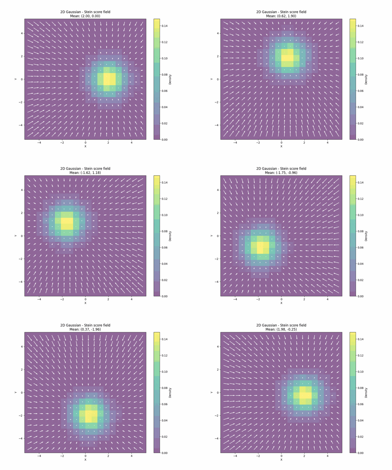
You can also see how the Stein score changes when we also change the covariance of the 2D gaussian:

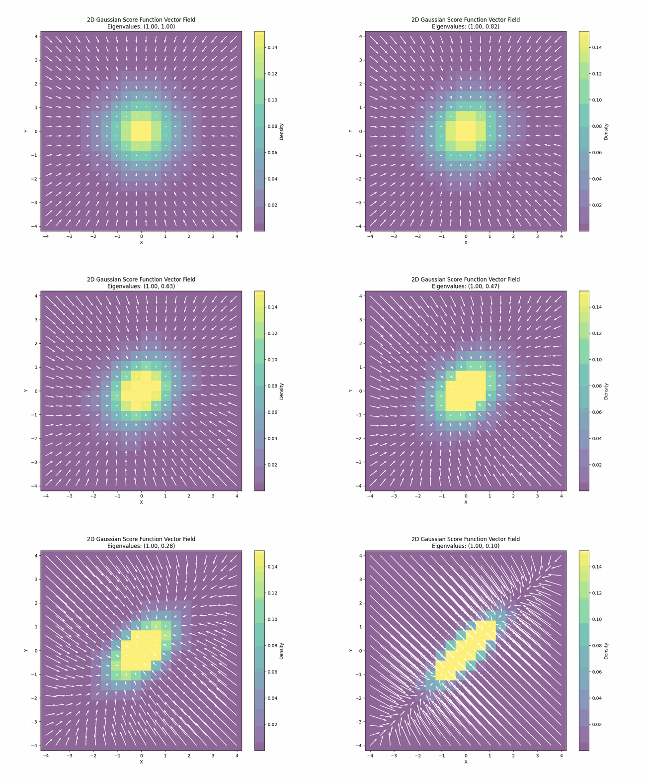
You can derive the closed-form Stein score function by just differentiating the log density or you can also learn it. There is a deep and fundamental connection between score matching/score estimation and diffusion models that I won’t go into details here but the main point is that this score can be learned from data.

For the sake of explanation and understanding, I will assume that we have data \(x \in \mathbb{R}^2\) and that this data is sampled from a 2D gaussian. The reason for this is that we can easily see what is going on, but do not limit your imagination to gaussians, the idea is to treat the score as a black box that could’ve been learned from the data.

The missing Stein metric tensor for the data manifold

The main question that we want to answer here is: how can we devise a metric tensor for the data manifold ?

This would be a very interesting metric tensor because it will allow us to compute distances between data samples, to compute geodesics between data samples, to measure angles in this data manifold, to compute inner products, etc.

One way to construct a metric tensor is to start from requirements that we need:

1. We need this metric tensor to contract space in the direction of the data (now you are starting to understand why the Stein score);
2. We want this metric tensor to be a Riemannian metric tensor (e.g. being positive definite), otherwise computing lengths and other properties becomes challenging;
3. The geodesics should be “attracted” or follow paths where the density (of data) is higher;

We have the Stein score function \(s(x)\) (which can also be learned \(s_{\theta}(x)\)) that gives us the direction to the data and is proportional to where we are in the data space. So we need to construct a metric tensor from this building block that would allow us to contract space in direction of data. One way to do that is to use the outer product:

$$ u \otimes v = uv^T $$

If we use the outer product of the Stein score with itself, in a \(x \in \mathbb{R}^2\) this will yield the following matrix:

$$ s(x) \otimes s(x) = \begin{bmatrix} s_1^2 & s_1 s_2 \\ s_2 s_1 & s_2^2 \end{bmatrix} $$

When we look from the matrix transformation perspective, when we transform a vector with this Stein score outer product (which is symmetric), we will get a transformation that will project the vector into the direction of the Stein score and it will scale the vector if the vector is parallel to the Stein score as you can see in the plot below:

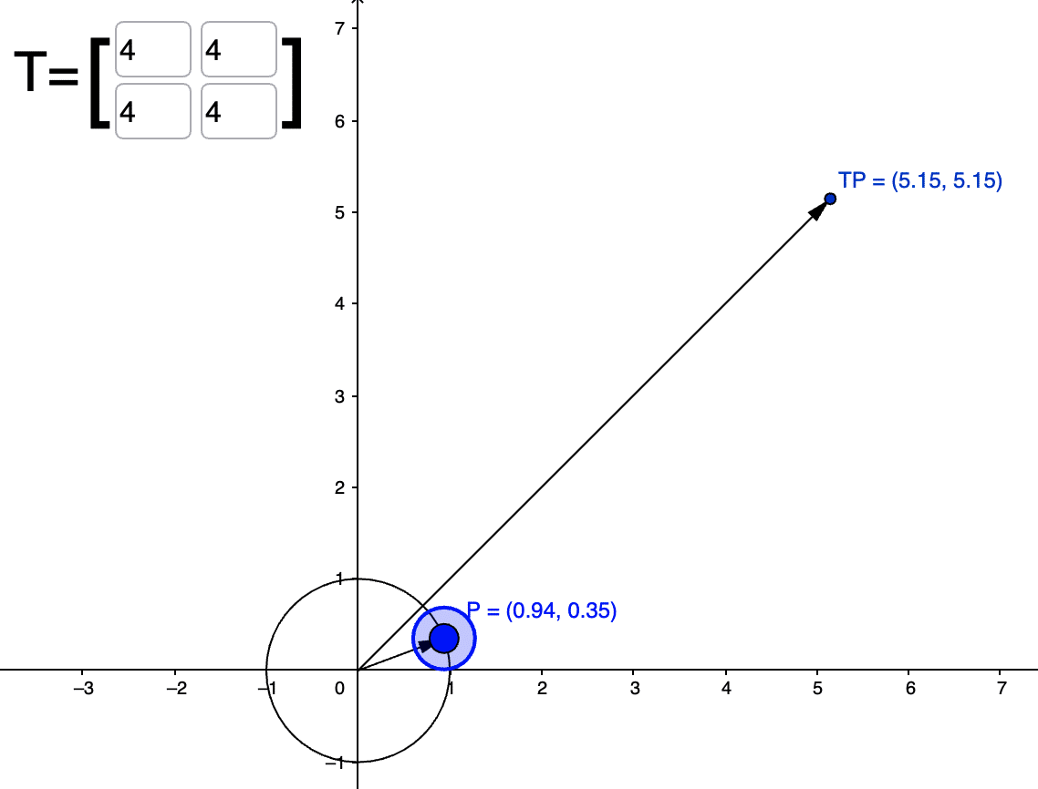
Where T is the outer product of the Stein score (\(s(x) = [2.0, 2.0]\)) and \(P\) is the vector we are transforming. You can see that the transformation result \(TP\) was projected along the direction of \(s(x)\) and scaled (the maximum scaling happens at when it is in exactly direction of the Stein score). Now, if we look at what happens when the vector is orthogonal to the Stein score you will see that there is contraction happening:

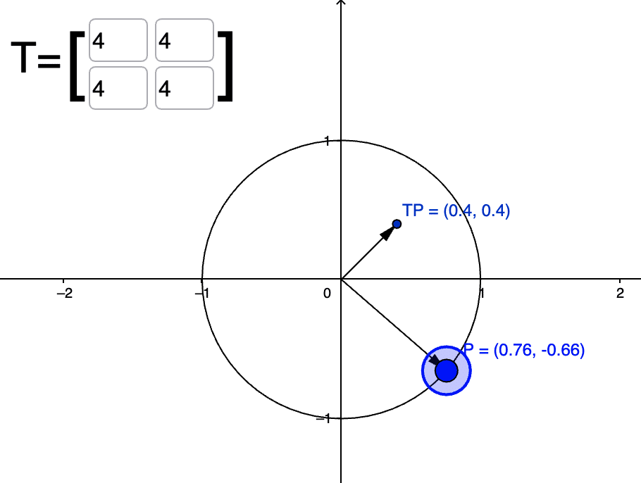
This is very helpful because it tells that we have a mechanism to contract the vector when it is orthogonal to the Stein score. But there is one problem: what we want is the opposite of this. One way to achieve this is to just invert the matrix as in:

$$ [s(x) \otimes s(x)]^{-1} $$

The problem is: outer products yield rank-1 matrices and we cannot invert rank-1 matrices as is. Now, if you read the first part of this article you are probably familiar with the Fisher information matrix and its use as a metric tensor in information geometry. The Fisher-Rao metric also uses the outer product:

$$ g_{ij} = \mathbb{E} \left[ \nabla_{\theta} \ln p(x | \theta) \otimes \nabla_{\theta} \ln p(x | \theta) \right] $$

However, what makes the rank-1 matrix be positive definite is the expectation over data because when you add a lot of directions in the outer product it becomes invertible and positive definite (under certain reasonable regularity assumptions of course).

Now, from the Bayesian perspective, the natural next step to do here would be to take expectation over the posterior, over the parameters of the model estimating the Score function (when learned) and that would probably make it positive definite. We can, however, adopt other approaches, one of them being “regularizing” the matrix, which in optimization is also called damping (please see Section 6 from K-FAC paper if you are interested), where add a small multiple of the identity matrix before inverting the matrix (as it is often done with the natural gradient). One interesting aspect is that if we just add the identity matrix we will get an interpolation between the Euclidean metric and the metric tensor that we are building that will contract the space in the direction of the Stein score, therefore yielding a very smooth interpolation between the two metric tensors. What I will do here is to add the identity matrix before taking the inverse and then we will see how it looks like, but be aware that you can also add a small multiple of the identity matrix and that will make contraction much stronger to the point of making geodesics going through singularities.

Here is what we have until now:

$$ g = [s(x) \otimes s(x) + I]^{-1} $$

Or if you are a Bayesian and want to integrate over the posterior (if you have a score model \(s_{\theta}(x)\) instead of a score function), then the metric tensor becomes the one below (which will propagate the uncertainty to the geodesics as well, which is quite amazing):

$$ g = \int_{\Theta} \left[ s_{\theta}(x) \otimes s_{\theta}(x) + I \right]^{-1} p(\theta \mid \mathcal{D}) \, d\theta $$

I’m calling it \(g\) because that is usually the name of the metric tensor in differential geometry. Let’s see how this transformation affects now a vector in the unity circle:

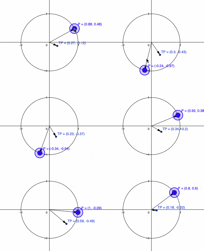
Now you can see that we are seeing the behavior that we wanted, it is contracting the vector \(P\) when it is in the direction of the Stein score while keeping it the same scale if it is orthogonal. There is one more thing we can do before we start using and analyzing this metric tensor \(g\), which is the efficient computation of the inverse.

Efficient inversion with Sherman-Morrison formula

The Sherman-Morrison formula equips us with a cheap way to compute the matrix inversion for rank-1 update to a matrix whose inverse has previously been computed:

$$ (A + u v^\top)^{-1} = A^{-1} – \frac{A^{-1} u v^\top A^{-1}}{1 + v^\top A^{-1} u} $$

In our case, since \(A = I\), \(A^{-1} = I\), \(u = s(x)\), and \(v^{\intercal} = s(x)^{\intercal}\), then we have this elegant formula for efficiently computing the metric tensor:

$$ g = I – \frac{s(x) s(x)^\top}{1 + \|s(x)\|^2} $$

This final formula ended up being similar to the Lorentz contraction, which is very interesting because we are also contracting length in the data manifold.

This metric tensor is very interesting because it basically defines the geometry of the data manifold so we can find geodesics in the data manifold, which are basically paths across data samples on the curved data manifold. The other interesting aspect of it is that it is telling us one very interesting aspect of score matching and score-based models (and also diffusion models): they are learning the building block of the metric tensor from the data manifold.

The fact that we can just plug the Stein score and efficiently compute the metric tensor for the data manifold is also very interesting because as I said earlier, there are multiple ways of computing or estimating the Stein score. This metric tensor puts the data as coordinates in the data manifold, just as the Fisher-Rao metric puts parameters as coordinates of the statistical manifold. I find this super exciting and with a lot of different connections with other concepts that could yield faster and high quality data samplers for score-based models, faster optimization algorithms, etc.

Now that we have our metric tensor \(g\) and we can compute it efficiently, let’s see some concrete cases of using it.

Optimizing geodesics on the data manifold

You can use many different parametrized curves but I will simplify here and use a discretization of a curve to find geodesics in the data manifold. To do that, I will use a path \(\gamma(t; \theta)\) that has multiple segments and then compute the energy \(E[\gamma]\) using the metric tensor \(g\) at each midpoint of these segments. Then we I’m going to do is to use Adam to minimize this energy and plot the animation of this procedure. What we want to do minimize the following objective:

$$ \theta^\ast = \arg \min_{\theta} E[\gamma_\theta] = \arg \min_{\theta} \left( \frac{1}{2} \int_{a}^{b} \langle \dot{\gamma}(t; \theta), \dot{\gamma}(t; \theta) \rangle_g \, dt \right) $$

Where we want to optimize the parameters of the discrete curve \(\gamma(t; \theta)\) to minimize the energy functional that we discussed in the introduction of this article. For the sake of example, I’m sampling from a 2D gaussian distribution that has a diagonal covariance matrix, so I can calculate the Stein score analytically and construct the metric tensor \(g\) with it. Keep in mind that just like I mentioned earlier, I’m using a parametric distribution but you can learn that from data and replace the Stein score with an estimator of it.

Deriving the Stein score from a multivariate Gaussian

It is often illuminating and interesting to look how the Stein score function looks like for Gaussians. The derivation can be a bit cumbersome but the end result is very simple.

1. Start from the definition of the Stein score:
   $$ \nabla_x \log p(x) $$
2. Take the gradient of the \(\log p(x)\) with respect to \(x\):
   $$\nabla_x \log p(x) = -\frac{1}{2} \nabla_x \left( (x – \mu)^\top \Sigma^{-1} (x – \mu) \right)$$
3. Expand the quadratic term:
   $$ (x – \mu)^\top \Sigma^{-1} (x – \mu) = \sum_{i,j} (x_i – \mu_i) \Sigma_{ij}^{-1} (x_j – \mu_j) $$
4. Differentiate with respect to \(x\):
   $$\nabla_x (x – \mu)^\top \Sigma^{-1} (x – \mu) = 2 \Sigma^{-1} (x – \mu)$$
5. And the Score function is:
   $$\nabla_x \log p(x) = -\Sigma^{-1} (x – \mu)$$

At the end the Score function is very simple, and it is even more illuminating when you think from a standard normal, that is simply \(\nabla_x \log p(x) = -\Sigma^{-1} x\), which is the inverse of the covariance matrix multiplied by \(x\). This basically scaling \(x\) according to the covariance of the distribution. If you are familiar with the Mahalanobis Distance, it is easy to see how you can rewrite it in terms of the Stein score.

Visualizing the Geodesic optimization (Energy minimization)

Now that we have the Sten score \(s(x) = \nabla_x \log p(x)\) we also have the metric tensor \(g\) as we defined earlier and we can then define a curve and optimize its parameters by minimizing the energy functional \(E[\gamma_\theta]\) where we compute the inner product using our derived metric tensor. Below you can see an animation of how this optimization looks like, this was done using a path with 60 points (the blue line). This path is initialized with a straight path between the two dots (green and yellow). This red straight line would be the shortest distance for the Euclidean metric, but as you will see, it is not the shortest distance in the data manifold. In the data manifold, the geodesic will bend towards the center of the Gaussian, where the data is, and therefore the shortest distance between two points is a curved geodesic and not a straight line anymore.

As you can see in the animation above, the path was bended to follow the curvature of the data, to pass through regions of space where there was contraction so that the energy and distances are lower through these paths.

Geodesics can start to get a bit non-intuitive when you have regions of high curvature as we can see below if we increase the correlation in the covariance matrix of the Gaussian and creating a more narrower distribution (showing anisotropy):

 

Note now how the path coming from the left is bending to take advantage of the curvature at the bottom of the plot and then we can see that the geodesic starts to be “attracted” by the regions of high data density. If we make the data follow even narrower distribution, you can clearly see the effects of anisotropy in the metric tensor:

Note that more at the end of the video you will be able to see that many segments of the path are being pulled to where the high data density is, this is happening because at that region of the space the space is highly compressed so the distances become smaller and therefore energy becomes lower, so the geodesic is trying to fit as many segments as possible in that region to reduce energy.

Understanding the Energy landscape

To understand why geodesics are following these paths, we can visualize the Energy landscape. It is quite tricky to visualize it since it depends on the direction of the displacement when computing the energy. We can, however, visualize the landscape for the initial position of the path (the red line shown above) and we can vary the data distribution to see how that changes energy: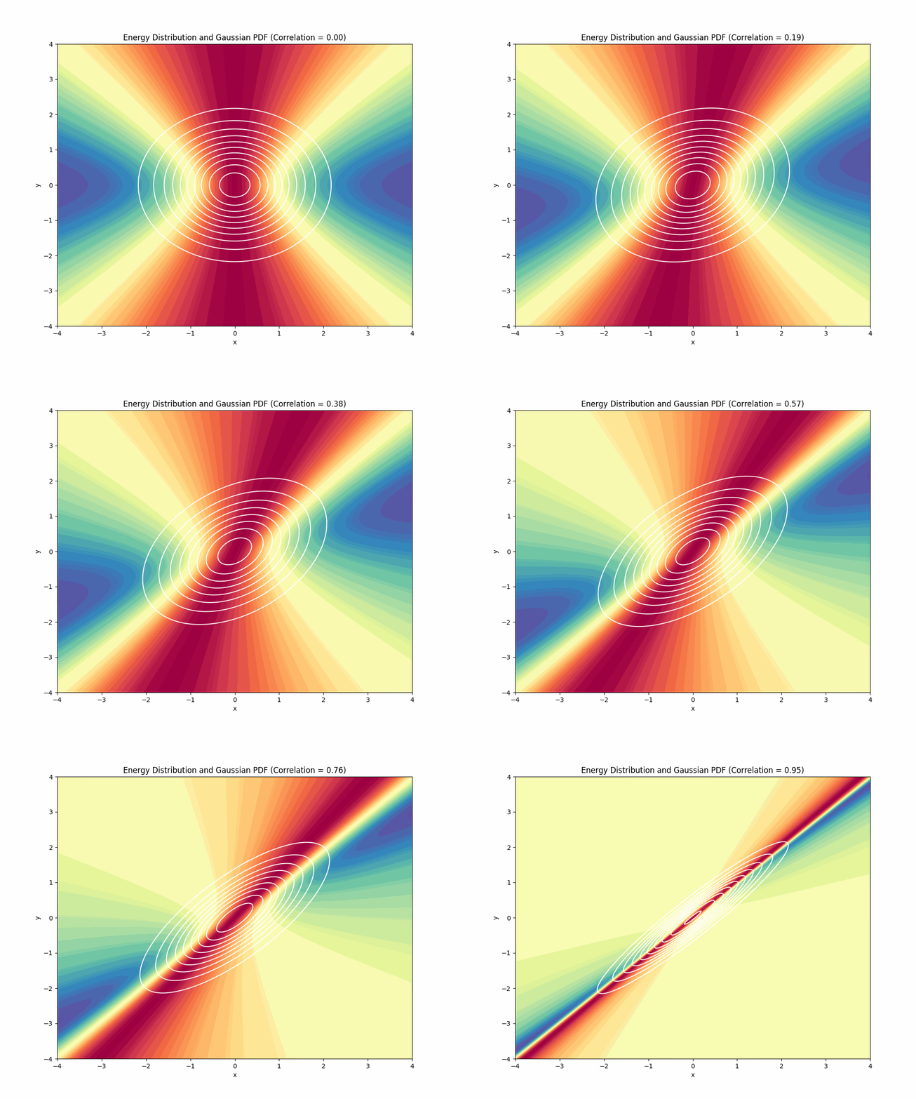

What we are visualizing in this animation above is the Energy at each point of the space:

$$ E[\gamma] = \int_0^1 \langle \dot{\gamma}(t), \dot{\gamma}(t) \rangle_g \, dt $$

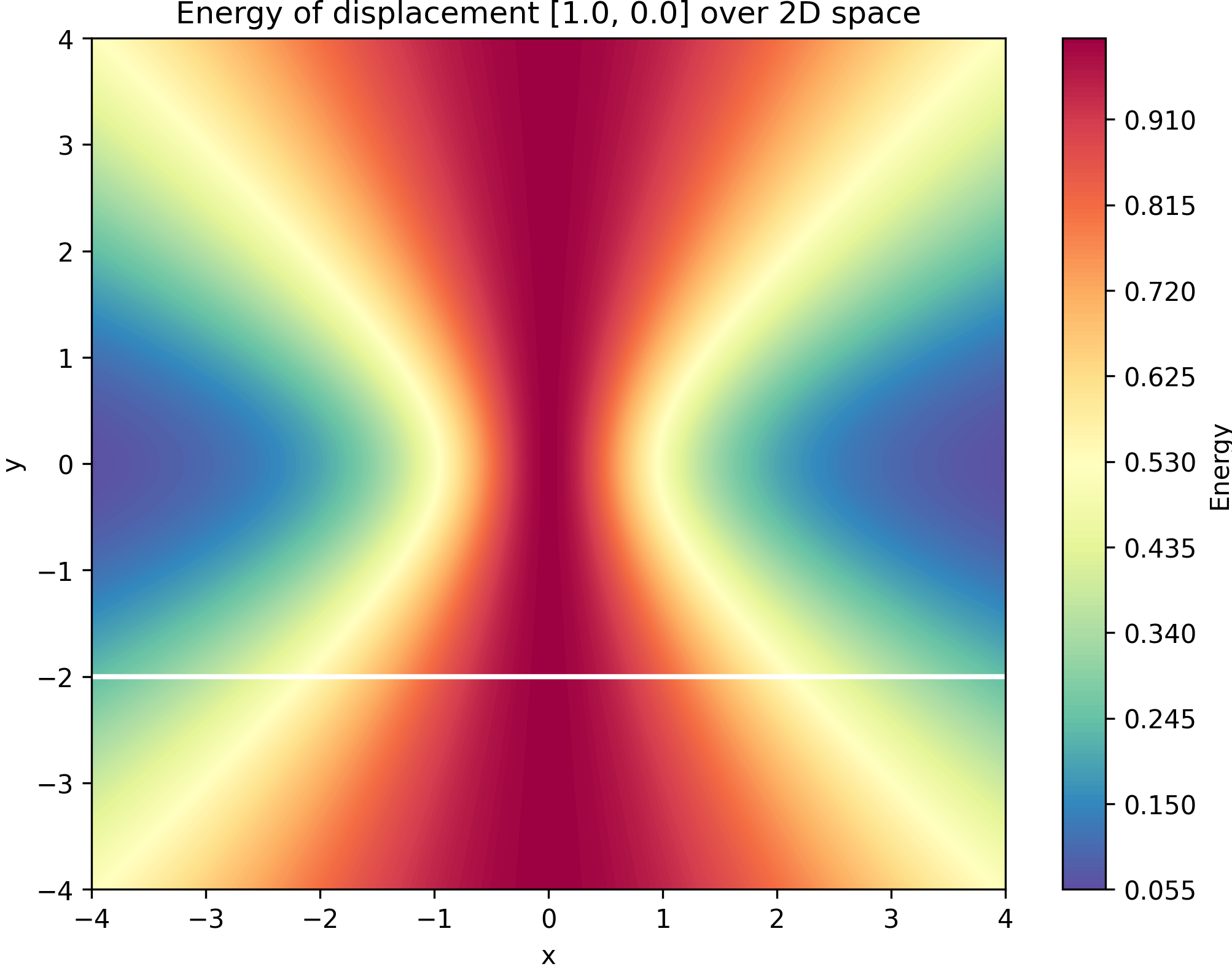
Note that we are using the path from -4 to 4 in the x-axis and fixing the y axis in -2 for the path (just as you can see in the red path shown in the animations we have shown earlier). Now you can understand why the path bends in the middle when we have a standard normal, you can see in the beginning of the animation that the Energy is higher (reds) exactly in the middle of the path, so the path bends that part to the center of the data to reduce its total energy. Please note that the displacement is zero in the y-axis because we are keeping the y dimension fixed. That’s the limitation of plotting it this way.

This is the energy landscape for a displacement of [1.0, 0.0], this is how the first step of optimization look like with the standard 2D gaussian (the white line is the path that we calculate the energy):

Now with the line over the energy heatmap you can clearly see why the middle of the line bent to the center, it is because the energy in the middle and below the 0 limit of the y-axis is much higher.

Some final thoughts

I hope you enjoyed this part II of the post, I will try to do a follow up soon with more uses of the metric tensor. One very interesting use would be in Langevin sampling, which seems very helpful because now that we have a metric tensor, we can use it in the Riemann Manifold Langevin Dynamics (RMLD). There are still A LOT of topics to explore with this metric tensor because it gives us a very important building block of the data manifold. You can also simplify a lot it by just using the diagonal of the metric tensor (as it is often done with the Fisher metric as well). I think that this metric tensor can help build more efficient sampling algorithms, provide manifold interpolations and help understand better our data manifolds. There are also very deep connections with diffusion and score-based generative models due to the building block we use to construct the metric tensor that I will be exploring more in the next part of this series. It is also important to note that there are also a lot of connections with physics as well as differential geometry is one of the most important frameworks used to model spacetime, so there is a lot to explore !

Changelog

17 Nov 2024: added more details abou the bayesian integration.

Citation