We are so used to Euclidean geometry that we often forget the importance of curved geometries and how to measure things that don’t live on orthonormal bases. Just like we cannot understand physics and spacetime curvature without Riemannian geometry, I don’t think we will ever get a deep understanding of Machine Learning (ML) or data without it. There are a lot of recent works that are more and more embedding (an overloaded term for this article) differential geometry into ML, but it is unfortunate that the term “geometric deep learning” ended up being a term that most people attach most of the time only to graphs. There is, however, a lot more than graphs in using modern geometry in ML.

I was reading the excellent article from Sander Dieleman about different perspectives on diffusion, so I thought it would be cool to try to contribute a bit with a new perspective.

A tale of two scores

Fisher information, metric and score

There are two important quantities that are widely known today and that keep popping out basically everywhere. The first one is the fisher information matrix \( \mathbf{F}\) (or FIM):

$$\mathbf{F}_\theta = \mathop{\mathbb{E}} \left[ \nabla_\theta \log p_\theta(y \vert x) \, \nabla_\theta \log p_\theta(y \vert x)^T \right] \,$$ with \(y \sim p_\theta (y \vert x)\) and \(x \sim p_{\text{data}}\). Note that where \(y\) comes from is very important and often a source of confusion. \(y\) is from the model’s predictive distribution (and this is quite interesting because it means you don’t need labels to estimate \( \mathbf{F}\) as well). The FIM is used in many places, such as Cramér-Rao bound, continual learning, posterior approximation, optimization, bayesian prior, KL divergence curvature, etc. Note that there is a lot of debate about the FIM vs empirical FIM and their different properties that I will skip going over here (I discussed this in the optimization context in this presentation if you are interested).

The fisher information matrix is also used in information geometry as a Riemannian metric where it is called Fisher-Rao metric (there are other names for it as well, which can be quite confusing). In this statistical manifold, where coordinates are parametrizing probability distributions, the metric (which equips the manifold) induces a inner product and allows us to compute norms and distances for distributions. Information geometry was pioneered by the late C. R. Rao and further developed and popularized by Shun-ichi Amari (who wrote some fine books about it).

We will talk more about the statistical manifold and what the metric actually does more intuitively later, but for now, note that the FIM uses the score, or what we can call, the Fisher score:

$$\mathbf{s}(\mathbf{\theta}) = \nabla_\mathbf{\theta} \log p(\mathbf{x} \vert \mathbf{\theta})$$

This score is the gradient of the log-likelihood w.r.t. its parameters \(\theta\), so it is telling us the steepness of the likelihood, with the FIM meaning the variance of this score. The FIM is also equivalent to the negative expectation of the Hessian matrix, which points its significance as a curvature at a parameter point, hence its appearance as a metric tensor as well (to be precise, as a metric tensor field).

The other score, as in score-based models (aka Stein score)

Now, there is another score, which is the one used in score-based models and score matching, which is often called Stein score:

$$\mathbf{s}(\mathbf{x}) = \nabla_{\mathbf{x}} \log p(\mathbf{x}\vert \mathbf{\theta})$$

Note that even though it looks similar and has a similar name to the previous score we showed, this is a very different score function. It doesn’t give you the gradients for distribution’s parameters but gradients w.r.t. data. It has been shown that we can estimate this score function from data even in absence of ground truths to this quantity. Yang Song has a nice article explaining motivation and recent developments.

The main point is that once you have this score function, you have a very powerful gradient field that tells you how samples should move in data space. You can then sample from the data distribution using Langevin sampling, which is basically SGD with noise to avoid collapse to a minima.

The missing metric

If the Fisher score gives the building block to the metric tensor for the statistical manifold, which metric can we build with this (Stein) score and which manifold does it belongs to ? It is surprising that we still don’t seem to have a clear formalization for this yet, at least I wasn’t able to find much about it. You can find some works about diffusion models on Riemannian manifolds but not about using the estimated (through modern deep learning models) score to build a Riemannian metric.

There is a nice quote from the physicist John Wheeler about Einstein’s relativity:

Space-time tells matter how to move and matter tells space-time how to curve.

– John Wheeler

It is very interesting that we can build a metric using this estimated score function, with the same mathematical framework used in the theory of relativity, where the quote can be modified to our case as:

Diffusion models tells data how to move and data tells Diffusion models how to curve.

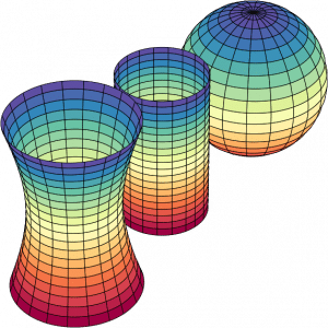
I will start to explore the topic with some examples in a series of posts, but here is a glimpse of a geodesic using the stein score as metric tensor where a Gaussian is curving the data manifold and creating this structure where the shortest distance from two points is not a straight line anymore:

This is a very interesting connection, seeing diffusion and score-based models as a metric tensor field can give us very interesting tools to explore data distances, geodesics, norms, etc, from the data manifold itself. We are still in the statistical domain, but the manifold is not the statistical manifold anymore where Riemannian coordinates parametrize distributions, it is a manifold where coordinates are the samples themselves. I think this connection of the score with the metric tensor field is a unexplored domain that is definitely very fertile, it can give us a much deeper understanding not only of data but also about our sampling algorithms.

The inner product induced by the score metric is the following:

$$\langle \delta_{P}, \delta_{Q} \rangle_{g_x}$$

where the metric tensor \(g_x\) is:

$$g_x = \nabla_{\mathbf{x}} \log p(\mathbf{x}\vert \mathbf{\theta})^{T} \nabla_{\mathbf{x}} \log p(\mathbf{x}\vert \mathbf{\theta})$$

So the inner product becomes:

$$\langle \delta_{P}, \delta_{Q} \rangle_{g_x} = \delta_{P} g_x \delta_{Q}$$

Note that we are using the (Stein) score as building block for our metric tensor \(g_x\), and this score is replaced by the estimated one parametrized by a deep neural network, so notation can become a nightmare because the base point where the metric tensor is evaluated is already used as lower index, so it can become \(g^{\theta}_x\) to denote that this metric tensor is parametrized by \(\theta\) (to make things worse, in diff geometry, indices positions also has an important meaning).

Hope you like the idea and please provide feedback and keep an eye in the next posts of this series.

Updates

27 Sept 2023: added more details about the metric tensor definition using the (Stein) score.

– Christian S. Perone