I had a spare M5stack that I got for a project and decided to repurpose it for a remote ML job monitor since it has a decent battery, an ESP32 + small keys and full keyboard + WiFi, it is starting to look cool:
Karl Popper offered an elegant normative account of science as a process of conjectures and refutations: we formulate hypotheses or theories, expose them to criticism, scrutiny and experiment, and retain only what survives our best attempts at falsification. Even though we couldn’t ever know if we reached the truth, we can approximate it and get closer to it, just like Popper noted from Xenophanes: “(…) for all is but a woven web of guesses.”. I really like Popper’s views on philosophy of science and also his work on political philosophy in “The Open Society and its Enemies” (1945) and I also wrote about some other aspects of his philosophy in relation to professional ethics here in the past as well, however, Popper’s philosophy helps describing this process of conjectures and refutations, but not the origin of genuinely novel hypotheses, and this is where many other philosophers like Thomas Kuhn (who proposed his “paradigm shift”) were closer on the account of how many scientific discoveries actually unfolded.
A few months ago NVIDIA open-sourced their Physical AI AV dataset (PAI) and since I was planning to experiment with developing the Flow Matching Elites after my earlier post on the Diffusion Elites, I decided to give it a try and use the NVIDIA PAI dataset for it instead of synthesizing trajectories.
NVIDIA PAI Dataset
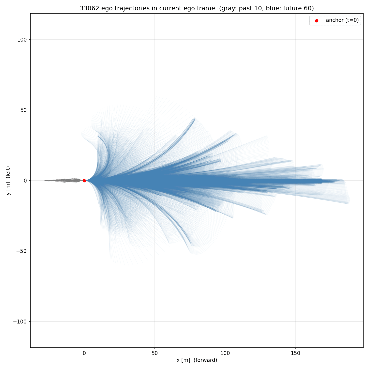
The NVIDIA PAI dataset seems to be mostly data collected using their Hyperion platform, not clear to me which versions of the platform they used (probably a mix) but since I was going to use only the ego motion trajectories I looked at some samples and they looked reasonable from the kinematic perspective (except for a few), since it is a lot of data with ~306k 20s scenes, I decided to use only ~20k initially to make training more amenable since I was using only a single RTX A6000 for the experiments.
Here you are some trajectories from the dataset after transforming into ego coordinate frame and interpolating at 10hz:
And here you are an animation sampling trajectories from it and unrolling to facilitate visualization:
Note that I’m not using anything from the dataset besides the ego motion trajectories, the main goal is to get a decent flow matching model where I can sample trajectories and then use this model in the elites loop like I showed on the Diffusion Elites post.
Flow Matching Elites
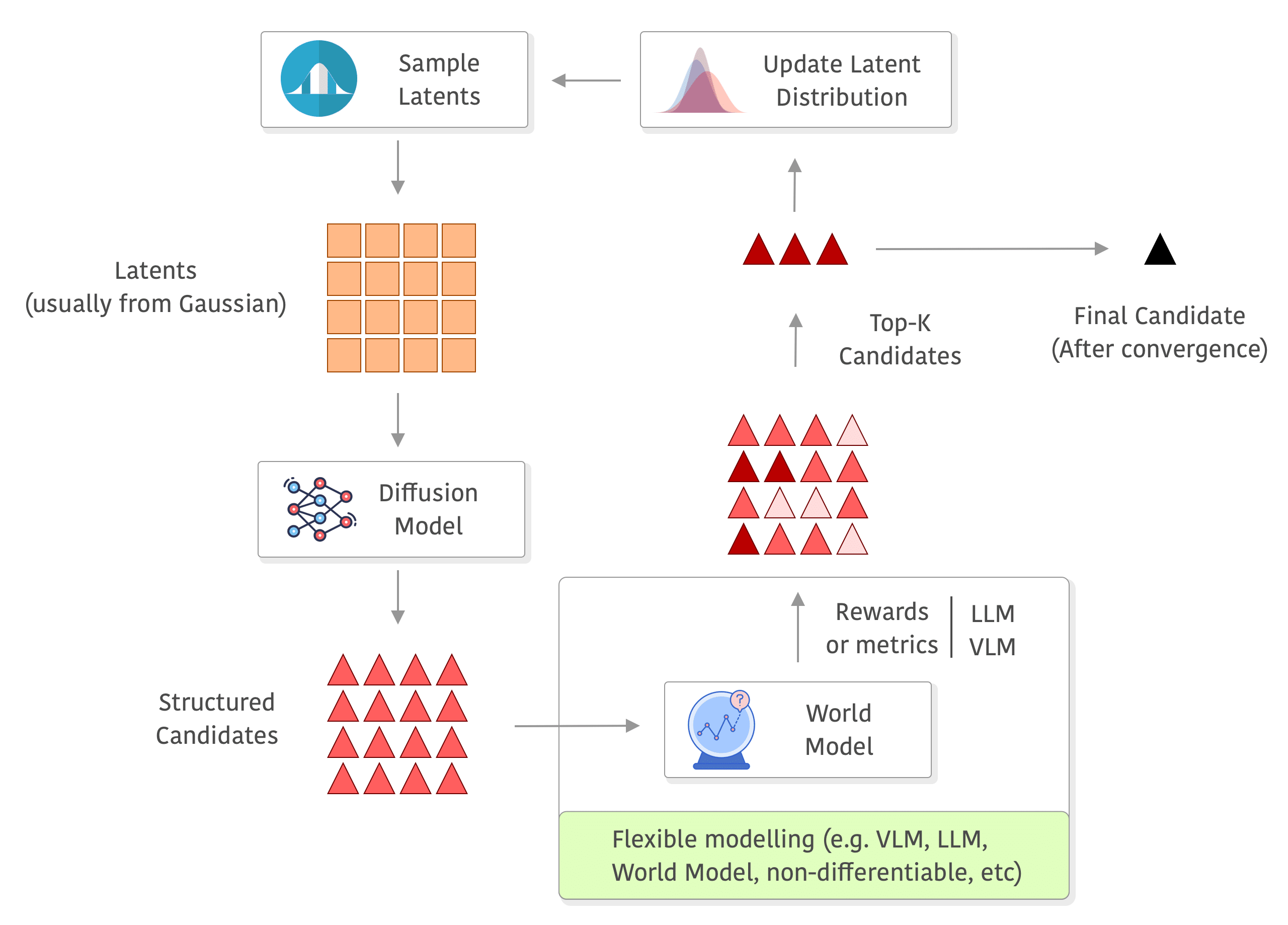
The diagram below shows the main overview of the method: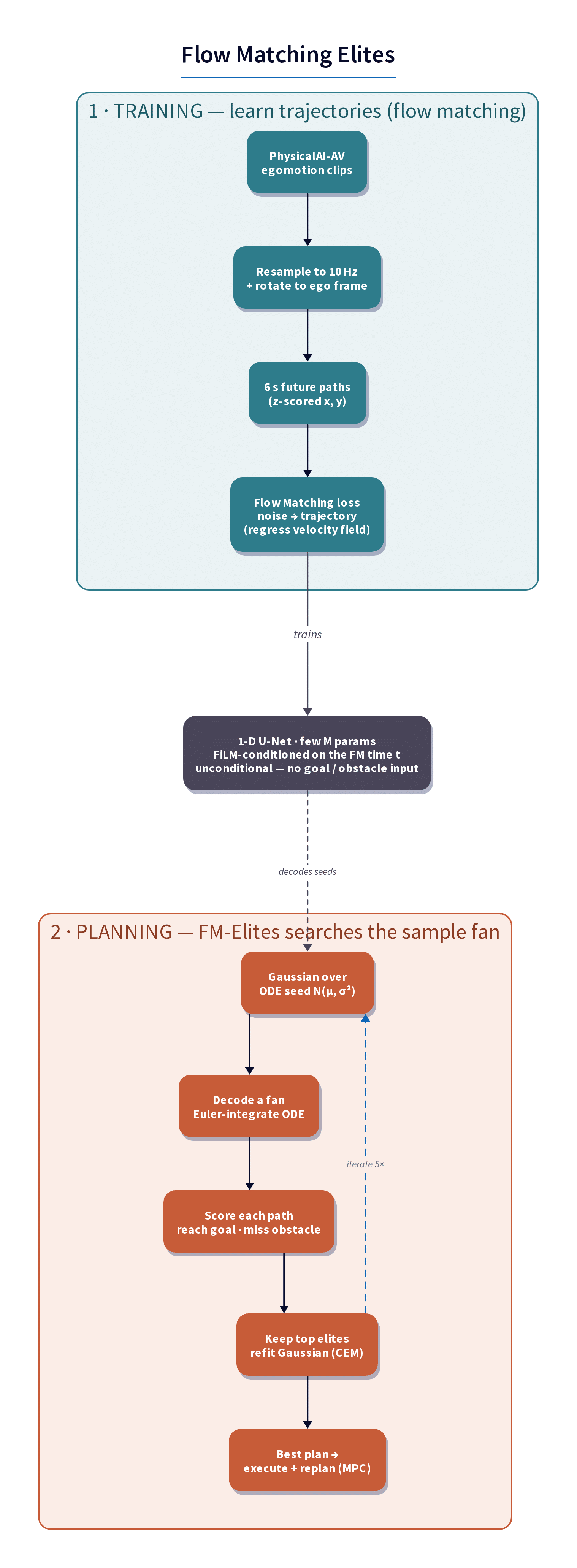
First we train a flow matching model using the 10hz resampled trajectories from the NVIDIA PAI dataset, we predict 6 seconds in the future unconditionally, there is no conditioning in the model other than the time conditioning from flow matching and we don’t use anything else from the dataset besides the ego trajectories.
The model I trained was a 1D CNN Unet using FiLM modulation for the time but no goal, obstacle or anything, we go from the gaussian noise to the trajectory unconditionally.
After that, we have a decent model where we can easily sample trajectories. This is where the Flow Matching Elites (FM-Elites) enters now, we basically run a few iteration steps of:
- Sampling from the unit Gaussian distribution
- Decode a bunch of trajectories using Euler for solving the flow matching ODE
- We then score the trajectories using a simple reward (distance to goal, obstacle avoidance and cross-tracking error)
- Then we keep the 10% elites and refit the Gaussian of the latent noise
- The best trajectory gets executed (first step or an action chunk)
- Repeat !
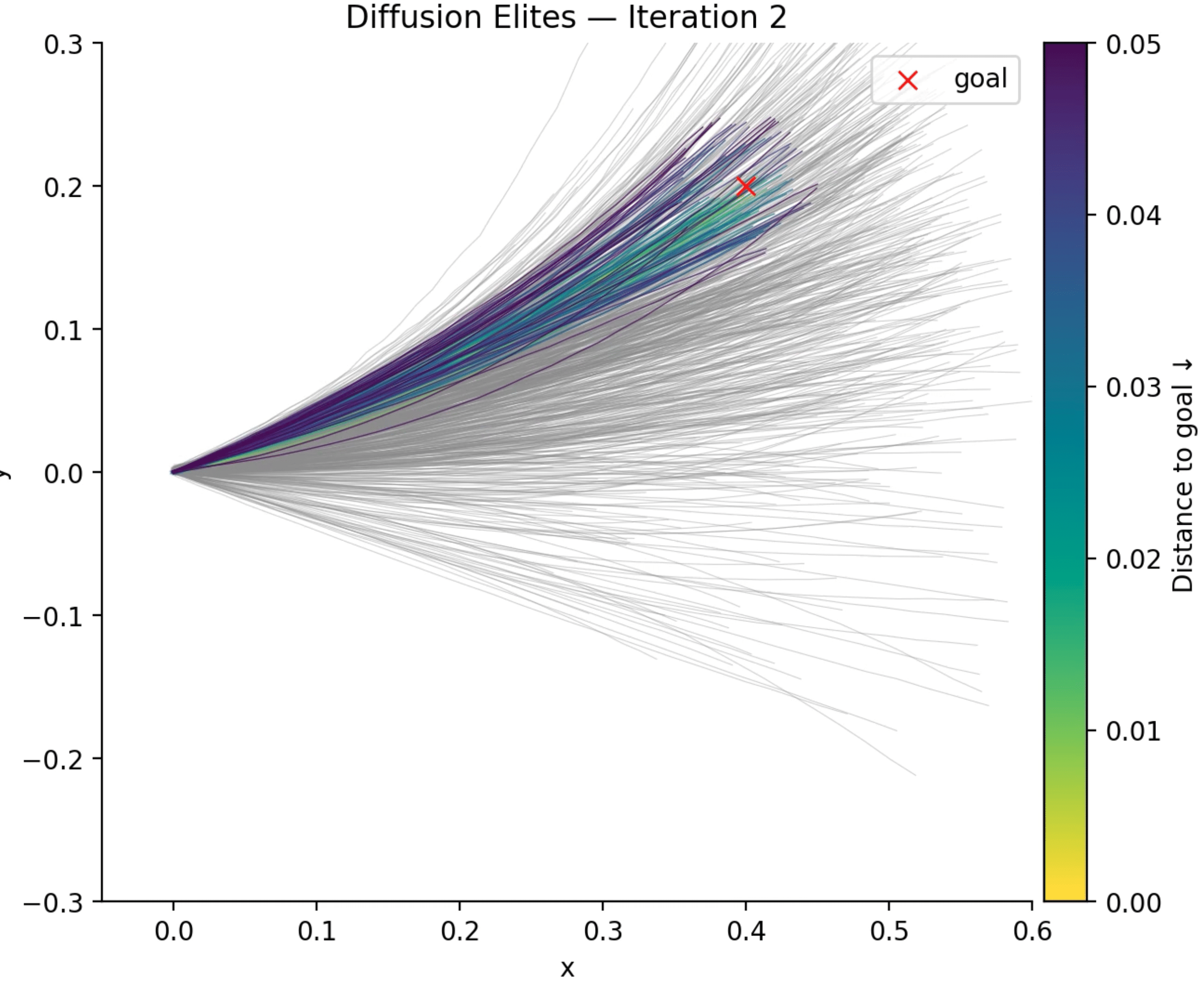
Some results with a random obstacle
The animation below shows the simulation when there is a static obstacle in front of the agent:
So there is a lot going on in this animation. First, note that the model is a unconditional model, doesn’t use a kinematic model and it doesn’t know about the existence of the obstacle as well, we are evolving the flow matching latents in order to adapt to the reward that we defined. The blue lines are all the candidates after the end of the inner-loop of the Flow Matching Elites and the orange one is the best candidate that was selected to be executed, this repeats every time there is a replanning, so Flow Matching Elites in this case is the inner-loop of the simulation. Note as well at the end when the agents gets closer to the target it has a lot of difficulty “touching” it, mainly because naturally the dataset doesn’t contain samples with the agent colliding so it is sampling low acceleration trajectories with stops, which is quite nice to see it naturally arising.
Now, what if the obstacle is moving ?
As we can see in the example above, it works just as fine as when it is static to find trajectories that are avoiding the safety margin of the obstacle as well.
These are just simple examples of using Flow Matching Elites for continuous control, but it is not the only task it can solve. The main interesting point here is that it is iterating on the flow matching latents (noise samples) using a population, so there are many knobs as well to improve and trade-off performance vs compute resources. I’m planning to open-source a framework that has a more general loop for experimenting with the algorithm, I think loops like that are very similar as well to what is being used for scientific discovery and I think there is a lot to explore there on other fields as well and also using more techniques from evolutionary computation (EC).
Hope you enjoyed !
– Christian S. Perone
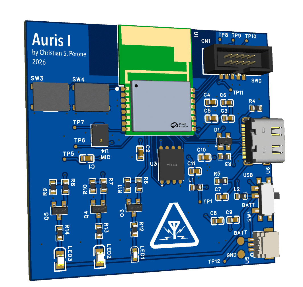
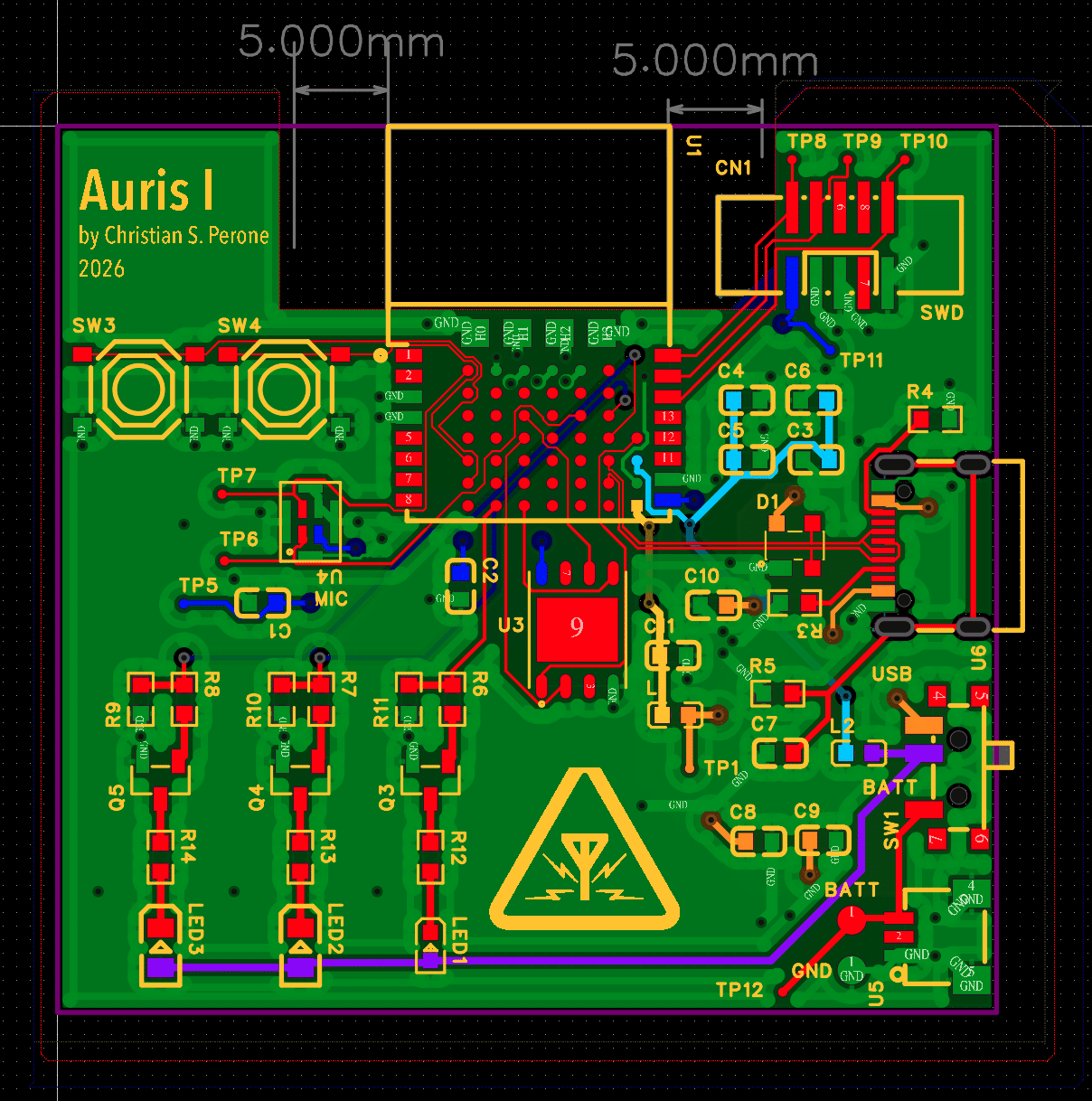
This short article is just to share a new side project I started working on during the 2025/2026 break. Over the past year, we have started to see a vast number of companies developing hardware for AI assistants. There were also a lot of acquisitions related to these devices (e.g., Amazon bought Bee [1]), and there were also a lot of fiascos, of course (e.g., Rabbit devices, Humane, and so on). I think that these devices have a strong future ahead due to their potential, so I started prototyping some code for recording, compression, and transmission, and testing some microphones. I found excellent transcription results even with a single microphone, so I decided to start a small side project which ended up becoming the the Auris I on the right.
Routing took quite a bit of work, as the main SoC used not only castellated pins but also pins under the chip which were very difficult to route. Another issue was the requirements of the RF module, which required some clearance on the ground plane, however, this was still much easier than going straight with the RF SoC without the guest board. The main challenges now are chip shortages for some components, but I expect to have a prototype working by the end of February. I will do another post then with more details and some interesting results. The board ended up being only 5 cm. There is, of course, a lot that can be reduced, but that will come in the Auris II after I manage to hack it a bit.
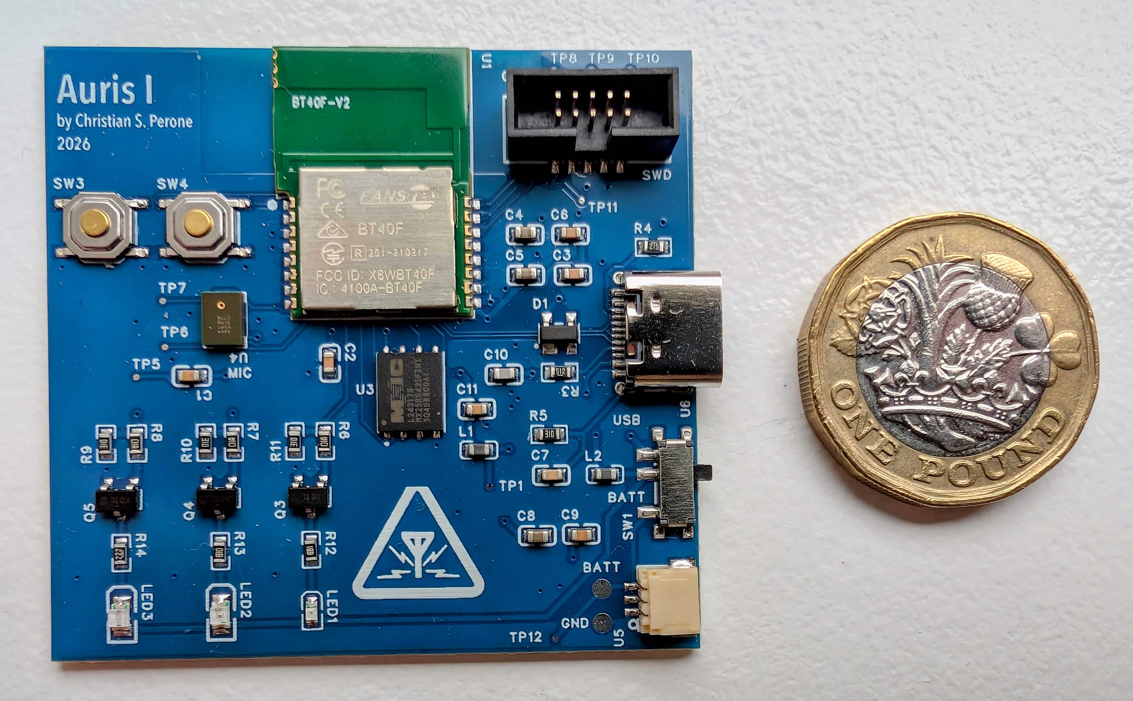
Update 7/Feb: Manufacturing, PCBs arrived !
I decided to go with JLCPCB with 4 layers as it is often quick and also very cheap, the only issue I faced was with the components, my board is based on nRF5340 (from Nordic Semiconductor) and modules with it were all without stock, so I had to acquire and wait for them to ship to JLCPCB, which took around 2 weeks. After that it was another week for the PCB fabrication and the assembly as well. Since the MEMS microphone was so small and the nRF5340 module also had pads under it, they required an x-ray inspection to make sure it was all connected fine. But that was around 4 pounds for x-ray and it was very fast as well. After around 5 days in total I finally received the PCBs and the quality is just amazing, I didn’t even order the cleaning of the board but they came all very clean well soldered as well.
I did all tests for the external flash, microphone, leds, battery/usb supply and also the SWD connection and it is all working fine, so now it is the fun part of coding, soon I will open-source everything, so stay tuned !
– Christian S. Perone
Hi everyone, just sharing some slides about Gemma3n architecture. I found Gemma3n a very interesting model so I decided to dig a bit further, given that information about it is still very scarce, hope you enjoy !
Download the slides PDF here.

Introduction
 It is not a secret that Diffusion models have become the workhorses of high-dimensionality generation: start with a Gaussian noise and, through a learned denoising trajectory, you get high-fidelity images, molecular graphs, or robot trajectories that look (uncannily) real. I wrote extensively about diffusion and its connection with the data manifold metric tensor recently as well, so if you are interested please take a look on it.
Now, for many engineering and practical tasks we care less about “looking real” and more about maximising a task-specific score or a reward from a simulator, a chemistry docking metric, a CLIP consistency score, human preference, etc. Even though we can use guidance or do a constrained sampling from the model, we often require differentiable functions for that. Evolution-style search methods (CEM, CMA-ES, etc), however, can shine in that regime, but naively applying them in the raw object space wastes most samples on absurd or invalid candidates and takes a lot of time to converge to a reasonable solution.
I have been experimenting on some personal projects with something that we can call “Diffusion Elites“, which aims to close this gap by letting a pre-trained diffusion model provide the prior and letting an adapted Cross-Entropy Method (CEM) steer the search inside its latent space instead. I found that this works quite well for many domains and it is also an impressively flexible method with a lot to explore (I will talk about some cases later).
To summarize, the method is as simple as the following:
- Draw a population of latent vectors from a Gaussian
- Run one full denoise pass to turn each latent into a structured object
- Score every object with any reward function
- Keep the top-K “elite” latents, refit a new Gaussian to them, and iterate
This five-line loop inherits the robust, gradient-free advantages of evolutionary search while guaranteeing that every candidate lives on the diffusion model’s data manifold. In practice that means fewer wasted evaluations, faster convergence, and dramatically higher-quality solutions for many tasks (e.g. planning, design, etc). In the rest of this post I will unpack the Diffusion Elites in detail, from the algorithm to some coding examples. Diffusion Elites shows that you can explore a diffusion model and turn it into a powerful black box optimizer, it is like doing search on the data manifold itself.
Diffusion Elites
Overview diagram
Below you can see a diagram of the process, I added a world model in the rewards to exemplify how you can use a world model and even do roll-outs there without any differentiability requirements, but you can really use anything to compute your rewards (e.g. you can also compute metrics on the outputs of the world model, or use a VLM/LLM as judge or even as world model as well):
I finally had some time over the holidays to complete the first panel of the TorchStation. The core idea is to have a monitor box that sits on your desk and tracks distributed model training. The panel shown below is a prototype for displaying GPU usage and memory. I’ll continue to post updates as I add more components. The main challenge with this board was power: the LED bars alone drew around 1.2A (when all full brightness and all lit up), so I had to use an external power supply and do a common ground with the MCU, for the panel I used a PLA Matte and 3mm. Wiring was the worst, this panel alone required at least 32 wires, but the panel will hide it quite well. I’m planning to support up to 8 GPUs per node, which aligns with the typical maximum found in many cloud instances. Here is the video, which was quite tricky to capture because of the camera metering of exposure that kept changing due to the LEDs (the video doesn’t do justice to how cool these LEDs are, they are very bright and clear even in daylight):
I’m using for the interface the Arduino Mega (which uses the ATmega2560) and Grove ports to make it easier to connect all of this, but I had to remove all VCCs from the ports to be able to supply from an external power supply, in the end it looks like this below:
                 ┌────────── PC USB (5V, ≤500 mA)
                 │
            +5 V │
                 ▼
     ┌─────────────────┐
     │  Arduino Mega   │  Data pins D2…D13, D66…D71 → LED bars
     └─────────────────┘
                ▲  GND (common reference)
                │
   ┌────────────┴──────────────┐
   │ 5V, ≥3 A switching PSU    │  ← external PSU
   └───────┬───────────┬───────┘
           │           │
           │ +5V       │ GND
           ▼           ▼
┌─────────────────────────────────┐
│ Grove Ports (VCC rail)          │ <– external 5V injected here
│ 8 × LED Bar cables              │
└─────────────────────────────────┘
PS: thanks for all the interest, here you are some discussions about VectorVFS as well:
Hacker News: discussion thread
Reddit: discussion thread
When I released EuclidesDB in 2018, which was the first modern vector database before milvus, pinecone, etc, I ended up still missing a piece of simple software for retrieval that can be local, easy to use and without requiring a daemon or any other sort of server and external indexes. After quite some time trying to figure it out what would be the best way to store embeddings in the filesystem I ended up in the design of VectorVFS.

The main goal of VectorVFS is to store the data embeddings (vectors) into the filesystem itself without requiring an external database. We don’t want to change the file contents as well and we also don’t want to create extra loose files in the filesystem. What we want is to store the embeddings on the files themselves without changing its data. How can we accomplish that ?
It turns out that all major Linux file systems (e.g. Ext4, Btrfs, ZFS, and XFS) support a feature that is called extended attributes (also known as xattr). This metadata is stored in the inode itself (ona reserved space at the end of each inode) and not in the data blocks (depending on the size). Some file systems might impose limits on the attributes, Ext4 for example requires them to be within a file system block (e.g. 4kb).
That is exactly what VectorVFS do, it embeds files (right now only images) using an encoder (Perception Encoder for the moment) and then it stores this embedding into the extended attributes of the file in the filesystem so we don’t need to create any other file for the metadata, the embedding will also be automatically linked directly to the file that was embedded and there is also no risks of this embedding being copied by mistake. It seems almost like a perfect solution for storing embeddings and retrieval that were there in many filesystems but it was never explored for that purpose before.
If you are interested, here is the documentation on how to install and use it, contributions are welcome !
