In 2009 I started playing with LLVM for some projects (data structure jit, for genetic programming, jit for tensorflow graphs, etc), and in these projects I realized how powerful LLVM design was at the time (and still is): using an elegant IR (intermediate representation) with an user-facing API and modularized front-ends and backends with plenty of transformation and optimization passes. Nowadays, LLVM is the main engine behind many compilers and JIT compilation and where most of the modern developments in compilers is happening.
On a related note, PyTorch is doing an amazing job of exposing more of the torch tracing system and its IR and graphs, not to mention their work on recent fusers and TorchDynamo. In this context, I was doing a small test to re-implement Shine, but using ATen ops for tensors and realized that there were not many educative tutorials on how to use LLVM to JIT PyTorch graphs, so this is a quick series (if time helps there will be more following posts) on how to use LLVM (python bindings) to go from PyTorch graphs (as traced by torch.fx) to LLVM IR and native code.
Detour – PyTorch NNC (Neural Net Compiler)
PyTorch itself also has a compiler that uses LLVM to generate native code for subgraphs that the fuser identifies. This is also called NNC (Neural Net Compiler) or Tensor Expressions (TE) as well, you can read more about them here in the C++ API tutorial. One thing to note though is that default binaries you get from PyTorch do not come linked to the LLVM libraries, so you need to compile it by yourself and enable LLVM backend, otherwise it won’t use LLVM to do the JIT compilation/optimization of the subgraphs. Let’s take a look at it first before starting our tutorial
These are the slides of the talk I presented on PyData Montreal on Feb 25th. It was a pleasure to meet you all ! Thanks a lot to Maria and Alexander for the invitation !
This is the post of 2020, so happy new year to you all !
I’m a huge fan of LLVM since 11 years ago when I started playing with it to JIT data structures such as AVLs, then later to JIT restricted AST trees and to JIT native code from TensorFlow graphs. Since then, LLVM evolved into one of the most important compiler framework ecosystem and is used nowadays by a lot of important open-source projects.
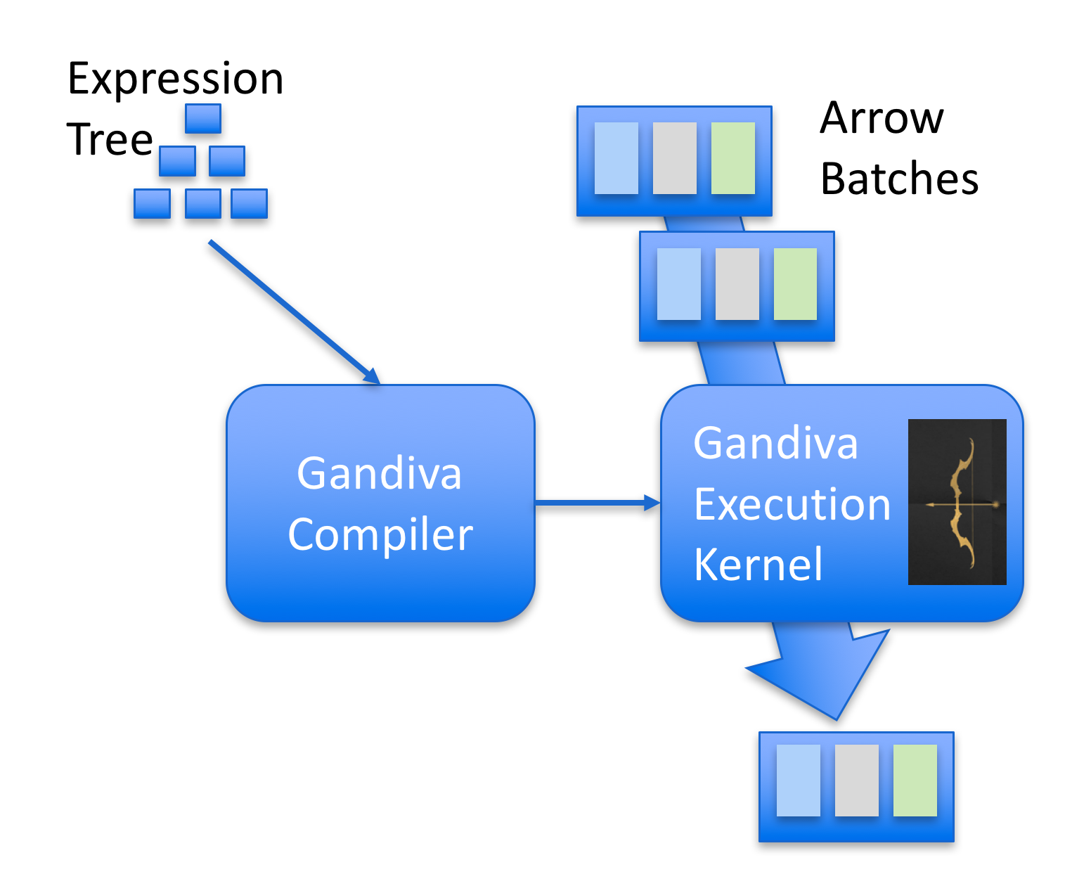
One cool project that I recently became aware of is Gandiva. Gandiva was developed by Dremio and then later donated to Apache Arrow (kudos to Dremio team for that). The main idea of Gandiva is that it provides a compiler to generate LLVM IR that can operate on batches of Apache Arrow. Gandiva was written in C++ and comes with a lot of different functions implemented to build an expression tree that can be JIT’ed using LLVM. One nice feature of this design is that it can use LLVM to automatically optimize complex expressions, add native target platform vectorization such as AVX while operating on Arrow batches and execute native code to evaluate the expressions.
The image below gives an overview of Gandiva:
An overview of how Gandiva works. Image from: https://www.dremio.com/announcing-gandiva-initiative-for-apache-arrow
In this post I’ll build a very simple expression parser supporting a limited set of operations that I will use to filter a Pandas DataFrame.
Building simple expression with Gandiva
In this section I’ll show how to create a simple expression manually using tree builder from Gandiva.
Using Gandiva Python bindings to JIT and expression
Before building our parser and expression builder for expressions, let’s manually build a simple expression with Gandiva. First, we will create a simple Pandas DataFrame with numbers from 0.0 to 9.0:
import pandas as pd
import pyarrow as pa
import pyarrow.gandiva as gandiva

# Create a simple Pandas DataFrame
df = pd.DataFrame({"x": [1.0 * i for i in range(10)]})
table = pa.Table.from_pandas(df)
schema = pa.Schema.from_pandas(df)
We converted the DataFrame to an Arrow Table, it is important to note that in this case it was a zero-copy operation, Arrow isn’t copying data from Pandas and duplicating the DataFrame. Later we get the schemafrom the table, that contains column types and other metadata.
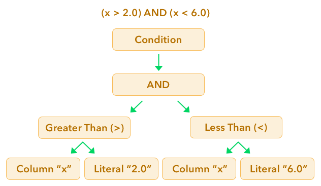
After that, we want to use Gandiva to build the following expression to filter the data:
(x > 2.0) and (x < 6.0)
This expression will be built using nodes from Gandiva:
builder = gandiva.TreeExprBuilder()

# Reference the column "x"
node_x = builder.make_field(table.schema.field("x"))

# Make two literals: 2.0 and 6.0
two = builder.make_literal(2.0, pa.float64())
six = builder.make_literal(6.0, pa.float64())

# Create a function for "x > 2.0"
gt_five_node = builder.make_function("greater_than",
                                     [node_x, two],
                                     pa.bool_())

# Create a function for "x < 6.0"
lt_ten_node = builder.make_function("less_than",
                                    [node_x, six],
                                    pa.bool_())
# Create an "and" node, for "(x > 2.0) and (x < 6.0)"
and_node = builder.make_and([gt_five_node, lt_ten_node])

# Make the expression a condition and create a filter
condition = builder.make_condition(and_node)
filter_ = gandiva.make_filter(table.schema, condition)
This code now looks a little more complex but it is easy to understand. We are basically creating the nodes of a tree that will represent the expression we showed earlier. Here is a graphical representation of what it looks like:
Inspecting the generated LLVM IR
Unfortunately, haven’t found a way to dump the LLVM IR that was generated using the Arrow’s Python bindings, however, we can just use the C++ API to build the same tree and then look at the generated LLVM IR:
auto field_x = field("x", float32());
auto schema = arrow::schema({field_x});

auto node_x = TreeExprBuilder::MakeField(field_x);

auto two = TreeExprBuilder::MakeLiteral((float_t)2.0);
auto six = TreeExprBuilder::MakeLiteral((float_t)6.0);

auto gt_five_node = TreeExprBuilder::MakeFunction("greater_than",
                                                  {node_x, two}, arrow::boolean());

auto lt_ten_node = TreeExprBuilder::MakeFunction("less_than",
                                                 {node_x, six}, arrow::boolean());

auto and_node = TreeExprBuilder::MakeAnd({gt_five_node, lt_ten_node});
auto condition = TreeExprBuilder::MakeCondition(and_node);

std::shared_ptr<Filter> filter;
auto status = Filter::Make(schema, condition, TestConfiguration(), &filter);
The code above is the same as the Python code, but using the C++ Gandiva API. Now that we built the tree in C++, we can get the LLVM Module and dump the IR code for it. The generated IR is full of boilerplate code and the JIT’ed functions from the Gandiva registry, however the important parts are show below:
As you can see, on the IR we can see the call to the functions less_than_float32_float_32 and greater_than_float32_float32that are the (in this case very simple) Gandiva functions to do float comparisons. Note the specialization of the function by looking at the function name prefix.
What is quite interesting is that LLVM will apply all optimizations in this code and it will generate efficient native code for the target platform while Godiva and LLVM will take care of making sure that memory alignment will be correct for extensions such as AVX to be used for vectorization.
This IR code I showed isn’t actually the one that is executed, but the optimized one. And in the optimized one we can see that LLVM inlined the functions, as shown in a part of the optimized code below:
You can see that the expression is now much simpler after optimization as LLVM applied its powerful optimizations and inlined a lot of Gandiva funcions.
Building a Pandas filter expression JIT with Gandiva
Now we want to be able to implement something similar as the Pandas’ DataFrame.query()function using Gandiva. The first problem we will face is that we need to parse a string such as (x > 2.0) and (x < 6.0), later we will have to build the Gandiva expression tree using the tree builder from Gandiva and then evaluate that expression on arrow data.
Now, instead of implementing a full parsing of the expression string, I’ll use the Python AST module to parse valid Python code and build an Abstract Syntax Tree (AST) of that expression, that I’ll be later using to emit the Gandiva/LLVM nodes.
The heavy work of parsing the string will be delegated to Python AST module and our work will be mostly walking on this tree and emitting the Gandiva nodes based on that syntax tree. The code for visiting the nodes of this Python AST tree and emitting Gandiva nodes is shown below:
As you can see, the code is pretty straightforward as I’m not supporting every possible Python expressions but a minor subset of it. What we do in this class is basically a conversion of the Python AST nodes such as Comparators and BinOps (binary operations) to the Gandiva nodes. I’m also changing the semantics of the & and the | operators to represent AND and OR respectively, such as in Pandas query()function.
Register as a Pandas extension
The next step is to create a simple Pandas extension using the gandiva_query() method that we created:
And that is it, now we can use this extension to do things such as:
df = pd.DataFrame({"a": [1.0 * i for i in range(nsize)]})
results = df.gandiva.query("a > 10.0")
As we have registered a Pandas extension called gandiva that is now a first-class citizen of the Pandas DataFrames.
Let’s create now a 5 million floats DataFrame and use the new query() method to filter it:
df = pd.DataFrame({"a": [1.0 * i for i in range(50000000)]})
df.gandiva.query("a < 4.0")

# This will output:
#     array([0, 1, 2, 3], dtype=uint32)
Note that the returned values are the indexes satisfying the condition we implemented, so it is different than the Pandas query()that returns the data already filtered.
I did some benchmarks and found that Gandiva is usually always faster than Pandas, however I’ll leave proper benchmarks for a next post on Gandiva as this post was to show how you can use it to JIT expressions.
That’s it ! I hope you liked the post as I enjoyed exploring Gandiva. It seems that we will probably have more and more tools coming up with Gandiva acceleration, specially for SQL parsing/projection/JITing. Gandiva is much more than what I just showed, but you can get started now to understand more of its architecture and how to build the expression trees.
Today, at the PyTorch Developer Conference, the PyTorch team announced the plans and the release of the PyTorch 1.0 preview with many nice features such as a JIT for model graphs (with and without tracing) as well as the LibTorch, the PyTorch C++ API, one of the most important release announcement made today in my opinion.
Given the huge interest in understanding how this new API works, I decided to write this article showing an example of many opportunities that are now open after the release of the PyTorch C++ API. In this post, I’ll integrate PyTorch inference into native NodeJS using NodeJS C++ add-ons, just as an example of integration between different frameworks/languages that are now possible using the C++ API.
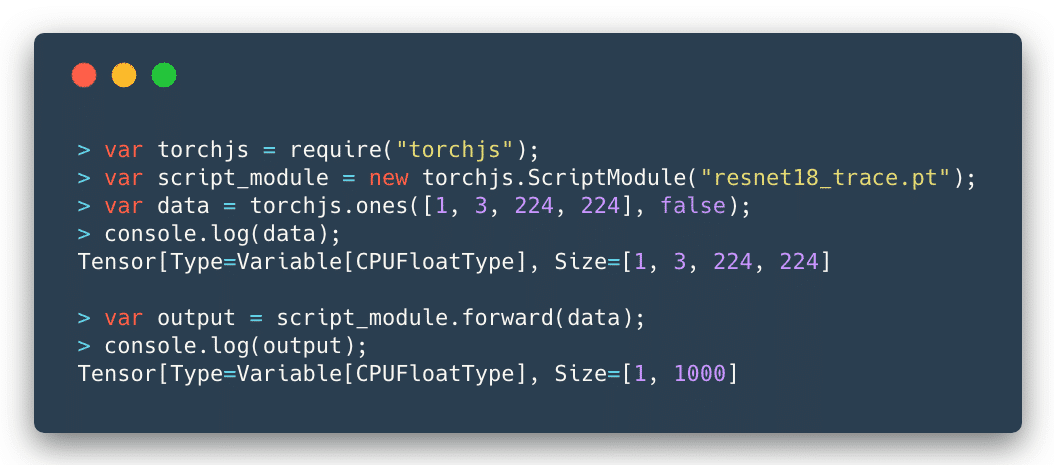
Below you can see the final result:
As you can see, the integration is seamless and I could use a traced ResNet as the computational graph model and feed any tensor to it to get the output predictions.
Introduction
Simply put, the libtorch is a library version of the PyTorch. It contains the underlying foundation that is used by PyTorch, such as the ATen (the tensor library), which contains all the tensor operations and methods. Libtorch also contains the autograd, which is the component that adds the automatic differentiation to the ATen tensors.
A word of caution for those who are starting now is to be careful with the use of the tensors that can be created both from ATen and autograd, do not mix them, the ATen will return the plain tensors (when you create them using the at namespace) while the autograd functions (from the torch namespace) will return Variable, by adding its automatic differentiation mechanism.
For a more extensive tutorial on how PyTorch internals work, please take a look on my previous tutorial on the PyTorch internal architecture.
Libtorch can be downloaded from the Pytorch website and it is only available as a preview for a while. You can also find the documentation in this site, which is mostly a Doxygen rendered documentation. I found the library pretty stable, and it makes sense because it is actually exposing the stable foundations of PyTorch, however, there are some issues with headers and some minor problems concerning the library organization that you might find while starting working with it (that will hopefully be fixed soon).
For NodeJS, I’ll use the Native Abstractions library (nan) which is the most recommended library (actually is basically a header-only library) to create NodeJS C++ add-ons and the cmake-js, because libtorch already provide the cmake files that make our building process much easier. However, the focus here will be on the C++ code and not on the building process.
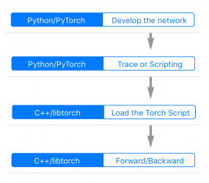
The flow for the development, tracing, serializing and loading the model can be seen in the figure on the left side.
It starts with the development process and tracing being done in PyTorch (Python domain) and then the loading and inference on the C++ domain (in our case in NodeJS add-on).
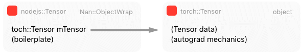
Wrapping the Tensor
In NodeJS, to create an object as a first-class citizen of the JavaScript world, you need to inherit from the ObjectWrap class, which will be responsible for wrapping a C++ component.
As you can see, most of the code for the definition of our Tensor class is just boilerplate. The key point here is that the torchjs::Tensor will wrap a torch::Tensor and we added two special public methods (setTensor and getTensor) to set and get this internal torch tensor.
I won’t show all the implementation details because most parts of it are NodeJS boilerplate code to construct the object, etc. I’ll focus on the parts that touch the libtorch API, like in the code below where we are creating a small textual representation of the tensor to show on JavaScript (toString method):
What we are doing in the code above, is just getting the internal tensor object from the wrapped object by unwrapping it. After that, we build a string representation with the tensor size (each dimension sizes) and its type (float, etc).
Wrapping Tensor-creation operations
Let’s create now a wrapper code for the torch::ones function which is responsible for creating a tensor of any defined shape filled with constant 1’s.
NAN_METHOD(ones) {
  // Sanity checking of the arguments
  if (info.Length() < 2)
    return Nan::ThrowError(Nan::New("Wrong number of arguments").ToLocalChecked());

  if (!info[0]->IsArray() || !info[1]->IsBoolean())
    return Nan::ThrowError(Nan::New("Wrong argument types").ToLocalChecked());

  // Retrieving parameters (require_grad and tensor shape)
  const bool require_grad = info[1]->BooleanValue();
  const v8::Local<v8::Array> array = info[0].As<v8::Array>();
  const uint32_t length = array->Length();

  // Convert from v8::Array to std::vector
  std::vector<long long> dims;
  for(int i=0; i<length; i++)
  {
    v8::Local<v8::Value> v;
    int d = array->Get(i)->NumberValue();
    dims.push_back(d);
  }

  // Call the libtorch and create a new torchjs::Tensor object
  // wrapping the new torch::Tensor that was created by torch::ones
  at::Tensor v = torch::ones(dims, torch::requires_grad(require_grad));
  auto newinst = Tensor::NewInstance();
  Tensor* obj = Nan::ObjectWrap::Unwrap<Tensor>(newinst);
  obj->setTensor(v);

  info.GetReturnValue().Set(newinst);
}
So, let’s go through this code. We are first checking the arguments of the function. For this function, we’re expecting a tuple (a JavaScript array) for the tensor shape and a boolean indicating if we want to compute gradients or not for this tensor node. After that, we’re converting the parameters from the V8 JavaScript types into native C++ types. Soon as we have the required parameters, we then call the torch::ones function from the libtorch, this function will create a new tensor where we use a torchjs::Tensor class that we created earlier to wrap it.
And that’s it, we just exposed one torch operation that can be used as native JavaScript operation.
Intermezzo for the PyTorch JIT
The introduced PyTorch JIT revolves around the concept of the Torch Script. A Torch Script is a restricted subset of the Python language and comes with its own compiler and transform passes (optimizations, etc).
This script can be created in two different ways: by using a tracing JIT or by providing the script itself. In the tracing mode, your computational graph nodes will be visited and operations recorded to produce the final script, while the scripting is the mode where you provide this description of your model taking into account the restrictions of the Torch Script.
Note that if you have branching decisions on your code that depends on external factors or data, tracing won’t work as you expect because it will record that particular execution of the graph, hence the alternative option to provide the script. However, in most of the cases, the tracing is what we need.
To understand the differences, let’s take a look at the Intermediate Representation (IR) from the script module generated both by tracing and by scripting.
@torch.jit.script
def happy_function_script(x):
    ret = torch.rand(0)
    if True == True:
        ret = torch.rand(1)
    else:
        ret = torch.rand(2)
    return ret

def happy_function_trace(x):
    ret = torch.rand(0)
    if True == True:
        ret = torch.rand(1)
    else:
        ret = torch.rand(2)
    return ret

traced_fn = torch.jit.trace(happy_function_trace,
                            (torch.tensor(0),),
                            check_trace=False)
In the code above, we’re providing two functions, one is using the @torch.jit.script decorator, and it is the scripting way to create a Torch Script, while the second function is being used by the tracing function torch.jit.trace. Not that I intentionally added a “True == True” decision on the functions (which will always be true).
Now, if we inspect the IR generated by these two different approaches, we’ll clearly see the difference between the tracing and scripting approaches:
As we can see, the IR is very similar to the LLVM IR, note that in the tracing approach, the trace recorded contains only one path from the code, the truth path, while in the scripting we have both branching alternatives. However, even in scripting, the always false branch can be optimized and removed with a dead code elimination transform pass.
PyTorch JIT has a lot of transformation passes that are used to do loop unrolling, dead code elimination, etc. You can find these passes here. Not that conversion to other formats such as ONNX can be implemented as a pass on top of this intermediate representation (IR), which is quite convenient.
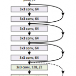
Tracing the ResNet
Now, before implementing the Script Module in NodeJS, let’s first trace a ResNet network using PyTorch (using just Python):
As you can see from the code above, we just have to provide a tensor example (in this case a batch of a single image with 3 channels and size 224×224. After that we just save the traced network into a file called resnet18_trace.pt.
Now we’re ready to implement the Script Module in NodeJS in order to load this file that was traced.
Wrapping the Script Module
This is now the implementation of the Script Module in NodeJS:
// Class constructor
ScriptModule::ScriptModule(const std::string filename) {
  // Load the traced network from the file
  this->mModule = torch::jit::load(filename);
}

// JavaScript object creation
NAN_METHOD(ScriptModule::New) {
  if (info.IsConstructCall()) {
    // Get the filename parameter
    v8::String::Utf8Value param_filename(info[0]->ToString());
    const std::string filename = std::string(*param_filename);

    // Create a new script module using that file name
    ScriptModule *obj = new ScriptModule(filename);
    obj->Wrap(info.This());
    info.GetReturnValue().Set(info.This());
  } else {
    v8::Local<v8::Function> cons = Nan::New(constructor);
    info.GetReturnValue().Set(Nan::NewInstance(cons).ToLocalChecked());
  }
}
As you can see from the code above, we’re just creating a class that will call the torch::jit::load function passing a file name of the traced network. We also have the implementation of the JavaScript object, where we convert parameters to C++ types and then create a new instance of the torchjs::ScriptModule.
The wrapping of the forward pass is also quite straightforward:
As you can see, in this code, we just receive a tensor as an argument, we get the internal torch::Tensor from it and then call the forward method from the script module, we wrap the output on a new torchjs::Tensor and then return it.
And that’s it, we’re ready to use our built module in native NodeJS as in the example below:
var torchjs = require("./build/Release/torchjs");
var script_module = new torchjs.ScriptModule("resnet18_trace.pt");
var data = torchjs.ones([1, 3, 224, 224], false);
var output = script_module.forward(data);
I hope you enjoyed ! Libtorch opens the door for the tight integration of PyTorch in many different languages and frameworks, which is quite exciting and a huge step towards the direction of production deployment code.
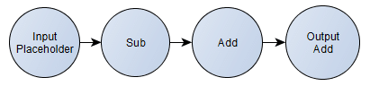
One of the most amazing components of the TensorFlow architecture is the computation graph that can be serialized using Protocol Buffers. This computation graph follows a well-defined format (click here for the proto files) and describes the computation that you specify (it can be a Deep Learning model like a CNN, a simple Logistic Regression or even any computation you want). For instance, here is an example of a very simple TensorFlow computation graph that we will use in this tutorial (using TensorFlow Python API):
As you can see, this is a very simple computation graph. First, we define the placeholder that will hold the input tensor and after that we specify the computation that should happen using this input tensor as input data. Here we can also see that we’re defining two important nodes of this graph, one is called “input” (the aforementioned placeholder) and the other is called “output“, that will hold the result of the final computation. This graph is the same as the following formula for a scalar: , where I intentionally added redundant operations to see LLVM constant propagation later.
In the last line of the code, we’re persisting this computation graph (including the constant values) into a serialized protobuf file. The final True parameter is to output a textual representation instead of binary, so it will produce the following human-readable output protobuf file (I omitted a part of it for brevity):
This is a very simple graph, and TensorFlow graphs are actually never that simple, because TensorFlow models can easily contain more than 300 nodes depending on the model you’re specifying, specially for Deep Learning models.
We’ll use the above graph to show how we can JIT native code for this simple graph using LLVM framework.
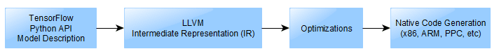
The LLVM Frontend, IR and Backend
The LLVM framework is a really nice, modular and complete ecosystem for building compilers and toolchains. A very nice description of the LLVM architecture that is important for us is shown in the picture below:
LLVM Compiler Architecture (AOSA/LLVM, Chris Lattner)
(The picture above is just a small part of the LLVM architecture, for a comprehensive description of it, please see the nice article from the AOSA book written by Chris Lattner)
Looking in the image above, we can see that LLVM provides a lot of core functionality, in the left side you see that many languages can write code for their respective language frontends, after that it doesn’t matter in which language you wrote your code, everything is transformed into a very powerful language called LLVM IR (LLVM Intermediate Representation) which is as you can imagine, a intermediate representation of the code just before the assembly code itself. In my opinion, the IR is the key component of what makes LLVM so amazing, because it doesn’t matter in which language you wrote your code (or even if it was a JIT’ed IR), everything ends in the same representation, and then here is where the magic happens, because the IR can take advantage of the LLVM optimizations (also known as transform and analysis passes).
After this IR generation, you can feed it into any LLVM backend to generate native code for any architecture supported by LLVM (such as x86, ARM, PPC, etc) and then you can finally execute your code with the native performance and also after LLVM optimization passes.
In order to JIT code using LLVM, all you need is to build the IR programmatically, create a execution engine to convert (during execution-time) the IR into native code, get a pointer for the function you have JIT’ed and then finally execute it. I’ll use here a Python binding for LLVM called llvmlite, which is very Pythonic and easy to use.
JIT’ing TensorFlow Graph using Python and LLVM
Let’s now use the LLVM and Python to JIT the TensorFlow computational graph. This is by no means a comprehensive implementation, it is very simplistic approach, a oversimplification that assumes some things: a integer closure type, just some TensorFlow operations and also a single scalar support instead of high rank tensors.
So, let’s start building our JIT code; first of all, let’s import the required packages, initialize some LLVM sub-systems and also define the LLVM respective type for the TensorFlow integer type:
from ctypes import CFUNCTYPE, c_int

import tensorflow as tf
from google.protobuf import text_format
from tensorflow.core.framework import graph_pb2
from tensorflow.core.framework import types_pb2
from tensorflow.python.framework import ops

import llvmlite.ir as ll
import llvmlite.binding as llvm

llvm.initialize()
llvm.initialize_native_target()
llvm.initialize_native_asmprinter()

TYPE_TF_LLVM = {
    types_pb2.DT_INT32: ll.IntType(32),
}
After that, let’s define a class to open the TensorFlow exported graph and also declare a method to get a node of the graph by name:
class TFGraph(object):
    def __init__(self, filename="graph.pb", binary=False):
        self.graph_def = graph_pb2.GraphDef()
        with open("graph.pb", "rb") as f:
            if binary:
                self.graph_def.ParseFromString(f.read())
            else:
                text_format.Merge(f.read(), self.graph_def)

    def get_node(self, name):
        for node in self.graph_def.node:
            if node.name == name:
                return node
And let’s start by defining our main function that will be the starting point of the code:
As you can see in the code above, we open the serialized protobuf graph and then get the input and output nodes of this graph. After that we also map the type of the both graph nodes (input/output) to the LLVM type (from TensorFlow integer to LLVM integer). We start then by defining a LLVM Module, which is the top level container for all IR objects. One module in LLVM can contain many different functions, here we will create just one function that will represent the graph, this function will receive as input argument the input data of the same type of the input node and then it will return a value with the same type of the output node.
After that we start by creating the entry block of the function and using this block we instantiate our IR Builder, which is a object that will provide us the building blocks for JIT’ing operations of TensorFlow graph.
Let’s now define the function that will do the real work of converting TensorFlow nodes into LLVM IR:
def build_graph(ir_builder, graph, node):
if node.op == "Add":
left_op_node = graph.get_node(node.input[0])
right_op_node = graph.get_node(node.input[1])
left_op = build_graph(ir_builder, graph, left_op_node)
right_op = build_graph(ir_builder, graph, right_op_node)
return ir_builder.add(left_op, right_op)
if node.op == "Sub":
left_op_node = graph.get_node(node.input[0])
right_op_node = graph.get_node(node.input[1])
left_op = build_graph(ir_builder, graph, left_op_node)
right_op = build_graph(ir_builder, graph, right_op_node)
return ir_builder.sub(left_op, right_op)
if node.op == "Placeholder":
function_args = ir_builder.function.args
for arg in function_args:
if arg.name == node.name:
return arg
raise RuntimeError("Input [{}] not found !".format(node.name))
if node.op == "Const":
llvm_const_type = TYPE_TF_LLVM[node.attr["dtype"].type]
const_value = node.attr["value"].tensor.int_val[0]
llvm_const_value = llvm_const_type(const_value)
return llvm_const_value
In this function, we receive by parameters the IR Builder, the graph class that we created earlier and the output node. This function will then recursively build the LLVM IR by means of the IR Builder. Here you can see that I only implemented the Add/Sub/Placeholder and Const operations from the TensorFlow graph, just to be able to support the graph that we defined earlier.
After that, we just need to define a function that will take a LLVM Module and then create a execution engine that will execute the LLVM optimization over the LLVM IR before doing the hard-work of converting the IR into native x86 code:
In the code above, you can see that we first get the CPU features (SSE, etc) into a list, after that we parse the LLVM IR from the module and then we create a engine using maximum optimization level (opt=3, roughly equivalent to the GCC -O3 parameter), we’re also printing the assembly code (in my case, the x86 assembly built by LLVM).
And here we just finish our run_main() function:
ret = build_graph(ir_builder, graph, output_node)
ir_builder.ret(ret)
with open("output.ir", "w") as f:
f.write(str(module))
engine = create_engine(module)
func_ptr = engine.get_function_address("tensorflow_graph")
cfunc = CFUNCTYPE(c_int, c_int)(func_ptr)
ret = cfunc(10)
print "Execution output: {}".format(ret)
As you can see in the code above, we just call the build_graph() method and then use the IR Builder to add the “ret” LLVM IR instruction (ret = return) to return the output of the IR function we just created based on the TensorFlow graph. We’re also here writing the IR output to a external file, I’ll use this LLVM IR file later to create native assembly for other different architectures such as ARM architecture. And finally, just get the native code function address, create a Python wrapper for this function and then call it with the argument “10”, which will be input data and then output the resulting output value.
And that is it, of course that this is just a oversimplification, but now we understand the advantages of having a JIT for our TensorFlow models.
The output LLVM IR, the advantage of optimizations and multiple architectures (ARM, PPC, x86, etc)
For instance, lets create the LLVM IR (using the code I shown above) of the following TensorFlow graph:
As you can see, the LLVM IR looks a lot like an assembly code, but this is not the final assembly code, this is just a non-optimized IR yet. Just before generating the x86 assembly code, LLVM runs a lot of optimization passes over the LLVM IR, and it will do things such as dead code elimination, constant propagation, etc. And here is the final native x86 assembly code that LLVM generates for the above LLVM IR of the TensorFlow graph:
As you can see, the optimized code removed a lot of redundant operations, and ended up just doing a add operation of 103, which is the correct simplification of the computation that we defined in the graph. For large graphs, you can see that these optimizations can be really powerful, because we are reusing the compiler optimizations that were developed for years in our Machine Learning model computation.
You can also use a LLVM tool called “llc”, that can take an LLVM IR file and the generate assembly for any other platform you want, for instance, the command-line below will generate native code for ARM architecture:
As you can see above, the ARM assembly code is also just a “add” assembly instruction followed by a return instruction.
This is really nice because we can take natural advantage of the LLVM framework. For instance, today ARM just announced the ARMv8-A with Scalable Vector Extensions (SVE) that will support 2048-bit vectors, and they are already working on patches for LLVM. In future, a really nice addition to LLVM would be the development of LLVM Passes for analysis and transformation that would take into consideration the nature of Machine Learning models.
And that’s it, I hope you liked the post ! Is really awesome what you can do with a few lines of Python, LLVM and TensorFlow.
Update 22 Aug 2016: TensorFlow team is actually working on a JIT (I don’t know if they are using LLVM, but it seems the most reasonable way to go in my opinion). In their paper, there is also a very important statement regarding Future Work that I cite here:
“We also have a number of concrete directions to improve the performance of TensorFlow. One such direction is our initial work on a just-in-time compiler that can take a subgraph of a TensorFlow execution, perhaps with some runtime profiling information about the typical sizes and shapes of tensors, and can generate an optimized routine for this subgraph. This compiler will understand the semantics of perform a number of optimizations such as loop fusion, blocking and tiling for locality, specialization for particular shapes and sizes, etc.” – TensorFlow White Paper
Full code
from ctypes import CFUNCTYPE, c_int
import tensorflow as tf
from google.protobuf import text_format
from tensorflow.core.framework import graph_pb2
from tensorflow.core.framework import types_pb2
from tensorflow.python.framework import ops
import llvmlite.ir as ll
import llvmlite.binding as llvm
llvm.initialize()
llvm.initialize_native_target()
llvm.initialize_native_asmprinter()
TYPE_TF_LLVM = {
types_pb2.DT_INT32: ll.IntType(32),
}
class TFGraph(object):
def __init__(self, filename="graph.pb", binary=False):
self.graph_def = graph_pb2.GraphDef()
with open("graph.pb", "rb") as f:
if binary:
self.graph_def.ParseFromString(f.read())
else:
text_format.Merge(f.read(), self.graph_def)
def get_node(self, name):
for node in self.graph_def.node:
if node.name == name:
return node
def build_graph(ir_builder, graph, node):
if node.op == "Add":
left_op_node = graph.get_node(node.input[0])
right_op_node = graph.get_node(node.input[1])
left_op = build_graph(ir_builder, graph, left_op_node)
right_op = build_graph(ir_builder, graph, right_op_node)
return ir_builder.add(left_op, right_op)
if node.op == "Sub":
left_op_node = graph.get_node(node.input[0])
right_op_node = graph.get_node(node.input[1])
left_op = build_graph(ir_builder, graph, left_op_node)
right_op = build_graph(ir_builder, graph, right_op_node)
return ir_builder.sub(left_op, right_op)
if node.op == "Placeholder":
function_args = ir_builder.function.args
for arg in function_args:
if arg.name == node.name:
return arg
raise RuntimeError("Input [{}] not found !".format(node.name))
if node.op == "Const":
llvm_const_type = TYPE_TF_LLVM[node.attr["dtype"].type]
const_value = node.attr["value"].tensor.int_val[0]
llvm_const_value = llvm_const_type(const_value)
return llvm_const_value
def create_engine(module):
features = llvm.get_host_cpu_features().flatten()
llvm_module = llvm.parse_assembly(str(module))
target = llvm.Target.from_default_triple()
target_machine = target.create_target_machine(opt=3, features=features)
engine = llvm.create_mcjit_compiler(llvm_module, target_machine)
engine.finalize_object()
print target_machine.emit_assembly(llvm_module)
return engine
def run_main():
    graph = TFGraph("graph.pb", False)
    input_node = graph.get_node("input")
    output_node = graph.get_node("output")

    input_type = TYPE_TF_LLVM[input_node.attr["dtype"].type]
    output_type = TYPE_TF_LLVM[output_node.attr["T"].type]

    module = ll.Module()
    func_type = ll.FunctionType(output_type, [input_type])
    func = ll.Function(module, func_type, name='tensorflow_graph')
    func.args[0].name = 'input'

    bb_entry = func.append_basic_block('entry')
    ir_builder = ll.IRBuilder(bb_entry)
ret = build_graph(ir_builder, graph, output_node)
ir_builder.ret(ret)

with open("output.ir", "w") as f:
    f.write(str(module))

engine = create_engine(module)

func_ptr = engine.get_function_address("tensorflow_graph")
cfunc = CFUNCTYPE(c_int, c_int)(func_ptr)
ret = cfunc(10)

print "Execution output: {}".format(ret)
if __name__ == "__main__":
run_main()
So I’m working on a Symbolic Regression Machine written in C/C++ called Shine, which is intended to be a JIT for Genetic Programming libraries (like Pyevolve for instance). The main rationale behind Shine is that we have today a lot of research on speeding Genetic Programming using GPUs (the GPU fever !) or any other special hardware, etc, however we don’t have many papers talking about optimizing GP using the state of art compilers optimizations like we have on clang, gcc, etc.
The “hot spot” or the component that consumes a lot of CPU resources today on Genetic Programming is the evaluation of each individual in order to calculate the fitness of the program tree. This evaluation is often executed on each set of parameters of the “training” set. Suppose you want to make a symbolic regression of a single expression like the Pythagoras Theorem and you have a linear space of parameters from 1.0 to 1000.0 with a step of 0.1 you have 10.000 evaluations for each individual (program tree) of your population !
What Shine does is described on the image below:
It takes the individual of the Genetic Programming engine and then converts it to LLVM Intermediate Representation (LLVM assembly language), after that it runs the transformation passes of the LLVM (here is where the true power of modern compilers enter on the GP context) and then the LLVM JIT converts the optimized LLVM IR into native code for the specified target (X86, PowerPC, etc).
You can see below the Shine architecture:
This architecture brings a lot of flexibility for Genetic Programming, you can for instance write functions that could be used later on your individuals on any language supported by the LLVM, what matters to Shine is the LLVM IR, you can use any language that LLVM supports and then use the IR generated by LLVM, you can mix code from C, C++, Ada, Fortran, D, etc and use your functions as non-terminal nodes of your Genetic Programming trees.
Shine is still on its earlier development, it looks a simple idea but I still have a lot of problems to solve, things like how to JIT the evaluation process itself instead of doing calls from Python using ctypes bindings of the JITed trees.
Doing Genetic Programming on the Python AST itself
During the development of Shine, an idea happened to me, that I could use a restricted Python Abstract Syntax Tree (AST) as the representation of individuals on a Genetic Programming engine, the main advantage of this is the flexibility and the possibility to reuse a lot of things. Of course that a shared library written in C/C++ would be useful for a lot of Genetic Programming engines that doesn’t uses Python, but since my spare time to work on this is becoming more and more rare I started to rethink the approach and use Python and the LLVM bindings for LLVM (LLVMPY) and I just discovered that is pretty easy to JIT a restricted set of the Python AST to native code using LLVM, and this is what this post is going to show.
JIT’ing a restricted Python AST
The most amazing part of LLVM is obviously the amount of transformation passes, the JIT and of course the ability to use the entire framework through a simple API (ok, not so simple sometimes). To simplify this example, I’m going to use an arbitrary restricted AST set of the Python AST that supports only subtraction (-), addition (+), multiplication (*) and division (/).
To understand the Python AST, you can use the Python parser that converts source into AST:
What the parse created was an Abstract Syntax Tree containing the BinOp (Binary Operation) with the left operator as the number 2, the right operator as the number 7 and the operation itself as Multiplication(Mult), very easy to understand. What we are going to do to create the LLVM IR is to create a visitor that is going to visit each node of the tree. To do that, we can subclass the Python NodeVisitor class from the ast module. What the NodeVisitor does is to visit each node of the tree and then call the method ‘visit_OPERATOR’ if it exists, when the NodeVisitor is going to visit the node for the BinOp for example, it will call the method ‘visit_BinOp’ passing as parameter the BinOp node itself.
The structure of the class for for the JIT visitor will look like the code below:
# Import the ast and the llvm Python bindings
import ast
from llvm import *
from llvm.core import *
from llvm.ee import *
import llvm.passes as lp

class AstJit(ast.NodeVisitor):
    def __init__(self):
        pass
What we need to do now is to create an initialization method to keep the last state of the JIT visitor, this is needed because we are going to JIT the content of the Python AST into a function and the last instruction of the function needs to return what was the result of the last instruction visited by the JIT. We also need to receive a LLVM Module object in which our function will be created as well the closure type, for the sake of simplicity I’m not type any object, I’m just assuming that all numbers from the expression are integers, so the closure type will be the LLVM integer type.
def __init__(self, module, parameters):
    self.last_state = None
    self.module = module
    # Parameters that will be created on the IR function
    self.parameters = parameters
    self.closure_type = Type.int()
    # An attribute to hold a link to the created function
    # so we can use it to JIT later
    self.func_obj = None
    self._create_builder()


def _create_builder(self):
    # How many parameters of integer type
    params = [self.closure_type] * len(self.parameters)

    # The prototype of the function, returning a integer
    # and receiving the integer parameters
    ty_func = Type.function(self.closure_type, params)

    # Add the function to the module with the name 'func_ast_jit'
    self.func_obj = self.module.add_function(ty_func, 'func_ast_jit')

    # Create an argument in the function for each parameter specified
    for index, pname in enumerate(self.parameters):
        self.func_obj.args[index].name = pname

    # Create a basic block and the builder
    bb = self.func_obj.append_basic_block("entry")
    self.builder = Builder.new(bb)
Now what we need to implement on our visitor is the ‘visit_OPERATOR’ methods for the BinOp and for the Numand Name operators. We will also implement the method to create the return instruction that will return the last state.
# A 'Name' is a node produced in the AST when you
# access a variable, like '2+x+y', 'x' and 'y' are
# the two names created on the AST for the expression.
def visit_Name(self, node):
    # This variable is what function argument ?
    index = self.parameters.index(node.id)
    self.last_state = self.func_obj.args[index]
    return self.last_state

# Here we create a LLVM IR integer constant using the
# Num node, on the expression '2+3' you'll have two
# Num nodes, the Num(n=2) and the Num(n=3).
def visit_Num(self, node):
    self.last_state = Constant.int(self.closure_type, node.n)
    return self.last_state

# The visitor for the binary operation
def visit_BinOp(self, node):
    # Get the operation, left and right arguments
    lhs = self.visit(node.left)
    rhs = self.visit(node.right)
    op = node.op

    # Convert each operation (Sub, Add, Mult, Div) to their
    # LLVM IR integer instruction equivalent
    if isinstance(op, ast.Sub):
        op = self.builder.sub(lhs, rhs, 'sub_t')
    elif isinstance(op, ast.Add):
        op = self.builder.add(lhs, rhs, 'add_t')
    elif isinstance(op, ast.Mult):
        op = self.builder.mul(lhs, rhs, 'mul_t')
    elif isinstance(op, ast.Div):
        op = self.builder.sdiv(lhs, rhs, 'sdiv_t')

    self.last_state = op
    return self.last_state

# Build the return (ret) statement with the last state
def build_return(self):
    self.builder.ret(self.last_state)
And that is it, our visitor is ready to convert a Python AST to a LLVM IR assembly language, to run it we’ll first create a LLVM module and an expression:
module = Module.new('ast_jit_module')
# Note that I'm using two variables 'a' and 'b'
expr = "(2+3*b+33*(10/2)+1+3/3+a)/2"
node = ast.parse(expr)
print ast.dump(node)
Now is when the real fun begins, we want to run LLVM optimization passes to optimize our code with an equivalent GCC -O2 optimization level, to do that we create a PassManagerBuilder and a PassManager, the PassManagerBuilder is the component that adds the passes to the PassManager, you can also manually add arbitrary transformations like dead code elimination, function inlining, etc:
pmb = lp.PassManagerBuilder.new()
# Optimization level
pmb.opt_level = 2

pm = lp.PassManager.new()
pmb.populate(pm)

# Run the passes into the module
pm.run(module)
print module
And here we have the optimized LLVM IR of the Python AST expression. The next step is to JIT that IR into native code and then execute it with some parameters:
And that’s it, you have created a AST->LLVM IR converter, optimized the LLVM IR with the transformation passes and then converted it to native code using the LLVM execution engine. I hope you liked =)
Following the recent article arguing why PyPy is the future of Python, I must say, PyPy is not the future of Python, is the present. When I have tested it last time (PyPy-c 1.1.0) with Pyevolve into the optimization of a simple Sphere function, it was at least 2x slower than Unladen Swallow Q2, but in that time, PyPy was not able to JIT. Now, with this new release of PyPy and the JIT’ing support, the scenario has changed.
PyPy has evolved a lot (actually, you can see this evolution here), a nice work was done on the GC system, saving (when compared to CPython) 8 bytes per object allocated, which is very interesting for applications that makes heavy use of object allocation (GP system are a strong example of this, since when they are implemented on object oriented languages, each syntax tree node is an object). Efforts are also being done to improve support for CPython extensions (written in C/C++), one of them is a little tricky: the use of RPyC, to proxy through TCP the remote calls to CPython; but the other seems by far more effective, which is the creation of the CPyExt subsystem. By using CPyExt, all you need is to have your CPython API functions implemented in CPyExt, a lot of people is working on this right now and you can do it too, it’s a long road to have a good API coverage, but when you think about advantages, this road becomes small.
In order to benchmark CPython, Jython, CPython+Psyco, Unladen Swallow and PyPy, I’ve used the Rastrigin function optimization (an example of that implementation is here in the Example 7 of Pyevolve 0.6rc1):
Due to its large search space and number of local minima, Rastrigin function is often used to measure the performance of Genetic Algorithms. Rastrigin function has a global minimum at where the ; in order to increase the search space and required resources, I’ve used 40 variables () and 10k generations.
Here are the information about versions used in this benchmark:
No warmup was performed in JVM or in PyPy. PyPy translator was executed using the “-Ojit” option in order to get the JIT version of the Python interpreter. The JVM was executed using the server mode, I’ve tested the client and server mode for Sun JVM and IcedTea6, the best results were observed from the server mode using Sun JVM, however when I’ve compared the client mode of IcedTea6 with the client mode of Sun JVM, the best results observed were from IcedTea6 (the same as using server mode in IcedTea6). Unladen Swallow was compiled using the project wiki instructions for building an optimized binary.
The machine used was an Intel(R) Core(TM) 2 Duo E4500 (2×2.20Ghz) with 2GB of RAM.
The result of the benchmark (measured using wall time) in seconds for each setup (these results are the best of 3 sequential runs):
As you can see, PyPy with JIT got a speedup of 2.57x when compared to CPython 2.6.5 and 2.0x faster than Unladen Swallow current trunk.
PyPy is not only the future of Python, but is becoming the present right now. PyPy will not bring us only an implementation of Python in Python (which in itself is the valuable result of great efforts), but also will bring the performance back (which many doubted at the beginning, wondering how could it be possible for an implementation of Python in Python be faster than an implementation in C ? And here is where the translation and JIT magic enters). When the time comes that Python interpreter can be entire written in a high level language (actually almost the same language, which is really weird), Python community can put their focus on improving the language itself instead of spending time solving the complexity of the lower level languages, is this not the great point of those efforts ?
By the way, just to note, PyPy isn’t only a translator for the Python interpreter written in RPython, it’s a translator of RPython, what means that PyPy isn’t only the future of Python, but probably, the future of many interpreters.
Hello folks, I always post about Python and EvoComp (Pyevolve), but this time it’s about C, LLVM, search algorithms and data structures. This post describes the efforts to implement an idea: to JIT (verb) algorithms and the data structures used by them, together.
AVL Tree Intro
Here is a short intro to AVL Trees from Wikipedia:
In computer science, an AVL tree is a self-balancing binary search tree, and it is the first such data structure to be invented. In an AVL tree, the heights of the two child subtrees of any node differ by at most one; therefore, it is also said to be height-balanced. Lookup, insertion, and deletion all take O(log n) time in both the average and worst cases, where n is the number of nodes in the tree prior to the operation. Insertions and deletions may require the tree to be rebalanced by one or more tree rotations.
The problem and the idea
When we have a data structure and algorithms to handle (insert, remove and lookup) that structure, the native code of our algorithm is usually full of overhead; for example, in an AVL Tree (Balanced Binary Tree), the overhead appear in: checking if we really have a left or right node while traversing the nodes for lookups, accessing nodes inside nodes, etc. This overhead creates unnecessary assembly operations which in turn, creates native code overhead, even when the compiler optimize it. This overhead directly impacts on the performance of our algorithm (this traditional approach, of course, give us a very flexible structure and the complexity (not Big-O) is easy to handle, but we pay for it: performance loss).
This website uses cookies to improve your experience. We'll assume you're ok with this, but you can opt-out if you wish. Cookie settingsACCEPT
Privacy & Cookies Policy
Privacy Overview
This website uses cookies to improve your experience while you navigate through the website. Out of these cookies, the cookies that are categorized as necessary are stored on your browser as they are essential for the working of basic functionalities of the website. We also use third-party cookies that help us analyze and understand how you use this website. These cookies will be stored in your browser only with your consent. You also have the option to opt-out of these cookies. But opting out of some of these cookies may have an effect on your browsing experience.
Necessary cookies are absolutely essential for the website to function properly. This category only includes cookies that ensures basic functionalities and security features of the website. These cookies do not store any personal information.
Any cookies that may not be particularly necessary for the website to function and is used specifically to collect user personal data via analytics, ads, other embedded contents are termed as non-necessary cookies. It is mandatory to procure user consent prior to running these cookies on your website.


-5)+100)") , where I intentionally added redundant operations to see LLVM constant propagation later.
, where I intentionally added redundant operations to see LLVM constant propagation later.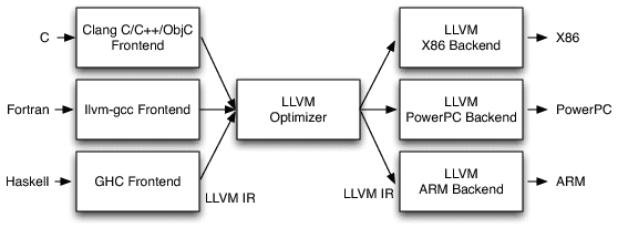


 = 10n + \sum_{i=1}^{n}{x_{i}^{2}}")
")

 where the
  = 0") ; in order to increase the search space and required resources, I’ve used 40 variables (
; in order to increase the search space and required resources, I’ve used 40 variables ( ) and 10k generations.

