We have been training language models (LMs) for years, but finding valuable resources about the data pipelines commonly used to build the datasets for training these models is paradoxically challenging. It may be because we often take it for granted that these datasets exist (or at least existed? As replicating them is becoming increasingly difficult). However, one must consider the numerous decisions involved in creating such pipelines, as it can significantly impact the final model’s quality, as seen recently in the struggle of models aiming to replicate LLaMA (LLaMA: Open and Efficient Foundation Language Models). It might be tempting to think that now, with large models that can scale well, data is becoming more critical than modeling, since model architectures are not radically changing much. However, data has always been critical.
This article provides a short introduction to the pipeline used to create the data to train LLaMA, but it allows for many variations and I will add details about other similar pipelines when relevant, such as RefinedWeb (The RefinedWeb Dataset for Falcon LLM: Outperforming Curated Corpora with Web Data, and Web Data Only) and The Pile (The Pile: An 800GB Dataset of Diverse Text for Language Modeling). This article is mainly based on the pipeline described in CCNet (CCNet: Extracting High Quality Monolingual Datasets from Web Crawl Data) and LLaMA’s paper, both from Meta. CCNet was developed focusing on the data source that is often the largest one, but also the most challenging in terms of quality: Common Crawl.
The big picture
The entire pipeline of CCNet (plus some minor modifications made by LLaMA’s paper) can be seen below. It has the following stages: data source, deduplication, language, filtering, and the “is-reference” filtering which was added in LLaMA. I will go through each one of them in the sections below.
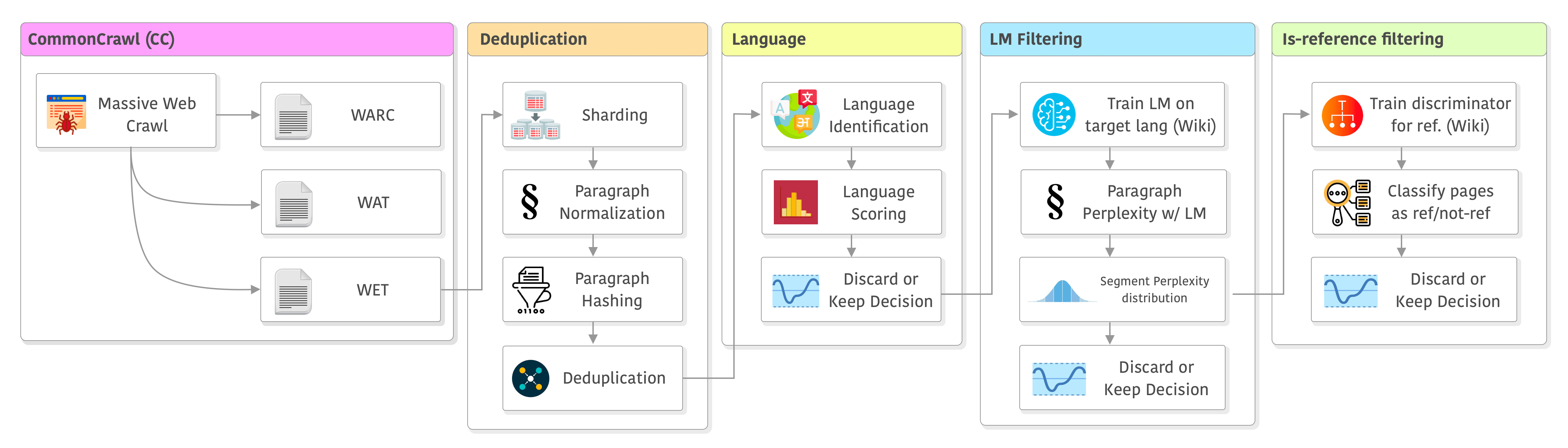
Let’s dive into it !

 , where the sum of all elements of the vector must equal 1. Softmax is used a lot in classification and I thought it would be interesting to visualize (when possible, on lower dimensions) the trajectories of individual samples in that simplex as predicted by the network while the network is being trained.