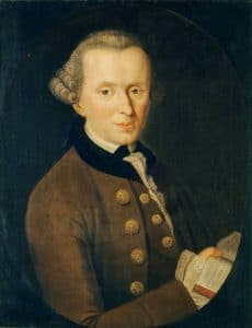
Portrait of Immanuel Kant by Johann Gottlieb Becker, 1768.
One of the most interesting, but also obscure and difficult parts of Kant’s critique is schematism. Every time I reflect on generalisation in Machine Learning and how concepts should be grounded, it always leads to the same central problem of schematism. Friedrich H. Jacobi said that schematism was “the most wonderful and most mysterious of all unfathomable mysteries and wonders …” [1], and Schopenhauer also said that it was “famous for its profound darkness, because nobody has yet been able to make sense of it” [1].
It is very rewarding, however, to realize that it is impossible to read Kant without relating much of his revolutionary philosophy to the difficult problems we are facing (and had always been) in AI, especially regarding generalisation. The first edition of the Critique of Pure Reason (CPR) was published more than 240 years ago, therefore historical context is often required to understand Kant’s writing, and to make things worse there is a lot of debate and lack of consensus among Kant’s scholars, however, even with these difficulties, it is still one of the most relevant and worth reading works of philosophy today.
Just sharing ~100 slides about PyTorch 2 internals focusing on recent innovations (Dynamo, Inductor, and ExecuTorch). I had a lot of fun preparing this and hope you’ll enjoy it. I’m planning to record it soon.
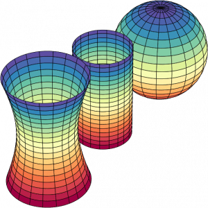
Different gaussian curvature surfaces. Image by Nicoguaro.
We are so used to Euclidean geometry that we often overlook the significance of curved geometries and the methods for measuring things that don’t reside on orthonormal bases. Just as understanding physics and the curvature of spacetime requires Riemannian geometry, I believe a profound comprehension of Machine Learning (ML) and data is also not possible without it. There is an increasing body of research that integrates differential geometry into ML. Unfortunately, the term “geometric deep learning” has predominantly become associated with graphs. However, modern geometry offers much more than just graph-related applications in ML.
I was reading the excellent article from Sander Dieleman about different perspectives on diffusion, so I thought it would be cool to try to contribute a bit with a new perspective.
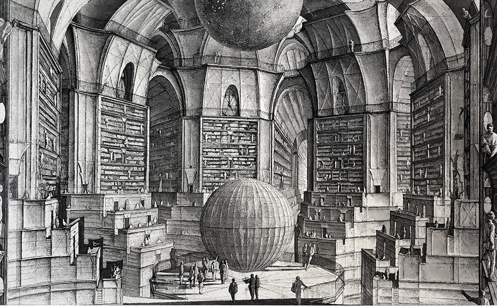
Erik Desmazieres’s “La Bibliothèque de Babel”. 1997.
We have been training language models (LMs) for years, but finding valuable resources about the data pipelines commonly used to build the datasets for training these models is paradoxically challenging. It may be because we often take it for granted that these datasets exist (or at least existed? As replicating them is becoming increasingly difficult). However, one must consider the numerous decisions involved in creating such pipelines, as it can significantly impact the final model’s quality, as seen recently in the struggle of models aiming to replicate LLaMA (LLaMA: Open and Efficient Foundation Language Models). It might be tempting to think that now, with large models that can scale well, data is becoming more critical than modeling, since model architectures are not radically changing much. However, data has always been critical.
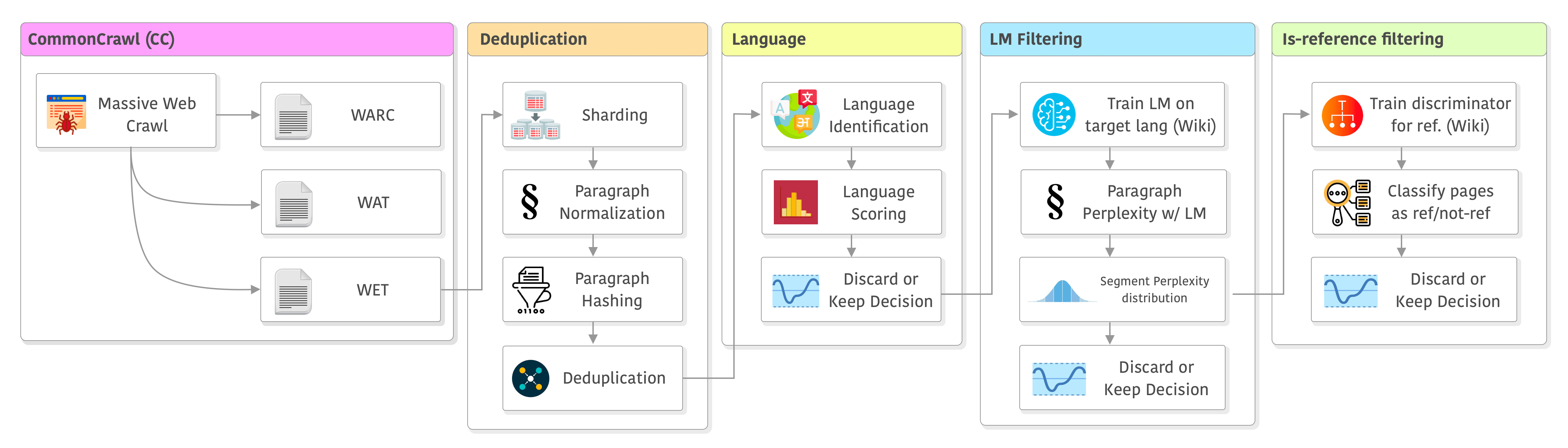
The entire pipeline of CCNet (plus some minor modifications made by LLaMA’s paper) can be seen below. It has the following stages: data source, deduplication, language, filtering, and the “is-reference” filtering which was added in LLaMA. I will go through each one of them in the sections below.
Visual overview of the CCNet pipeline with some modifications done in LLaMA. Click to enlarge.
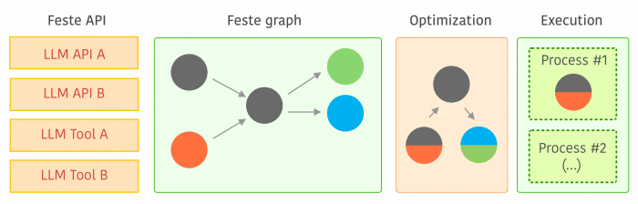
I just released Feste, a free and open-source framework with a permissive license that allows scalable composition of NLP tasks using a graph execution model that is optimized and executed by specialized schedulers. The main idea behind Feste is that it builds a graph of execution instead of executing tasks immediately, this graph allows Feste to optimize and parallelize it. One main example of optimization is when we have multiple calls to the same backend (e.g. same API), Feste automatically fuses these calls into a single one and therefore it batches the call to reduce latency and improve backend inference leverage of GPU vectorization. Feste also executes tasks that can be done in parallel in different processes, so the user doesn’t have to care about parallelization, especially when there are multiple frameworks using different concurrency strategies.
Training neural networks is often done by measuring many different metrics such as accuracy, loss, gradients, etc. This is most of the time done aggregating these metrics and plotting visualizations on TensorBoard.
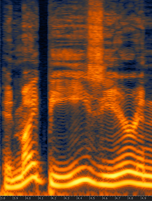
There are, however, other senses that we can use to monitor the training of neural networks, such as sound. Sound is one of the perspectives that is currently very poorly explored in the training of neural networks. Human hearing can be very good a distinguishing very small perturbations in characteristics such as rhythm and pitch, even when these perturbations are very short in time or subtle.
For this experiment, I made a very simple example showing a synthesized sound that was made using the gradient norm of each layer and for step of the training for a convolutional neural network training on MNIST using different settings such as different learning rates, optimizers, momentum, etc.
You’ll need to install PyAudio and PyTorch to run the code (in the end of this post).
Training sound with SGD using LR 0.01
This segment represents a training session with gradients from 4 layers during the first 200 steps of the first epoch and using a batch size of 10. The higher the pitch, the higher the norm for a layer, there is a short silence to indicate different batches. Note the gradient increasing during time.
Training sound with SGD using LR 0.1
Same as above, but with higher learning rate.
Training sound with SGD using LR 1.0
Same as above, but with high learning rate that makes the network to diverge, pay attention to the high pitch when the norms explode and then divergence.
Training sound with SGD using LR 1.0 and BS 256
Same setting but with a high learning rate of 1.0 and a batch size of 256. Note how the gradients explode and then there are NaNs causing the final sound.
Training sound with Adam using LR 0.01
This is using Adam in the same setting as the SGD.
Source code
For those who are interested, here is the entire source code I used to make the sound clips:
import pyaudio
import numpy as np
import wave

import torch
import torch.nn as nn
import torch.nn.functional as F
import torch.optim as optim
from torchvision import datasets, transforms


class Net(nn.Module):
    def __init__(self):
        super(Net, self).__init__()
        self.conv1 = nn.Conv2d(1, 20, 5, 1)
        self.conv2 = nn.Conv2d(20, 50, 5, 1)
        self.fc1 = nn.Linear(4*4*50, 500)
        self.fc2 = nn.Linear(500, 10)

        self.ordered_layers = [self.conv1,
                               self.conv2,
                               self.fc1,
                               self.fc2]

    def forward(self, x):
        x = F.relu(self.conv1(x))
        x = F.max_pool2d(x, 2, 2)
        x = F.relu(self.conv2(x))
        x = F.max_pool2d(x, 2, 2)
        x = x.view(-1, 4*4*50)
        x = F.relu(self.fc1(x))
        x = self.fc2(x)
        return F.log_softmax(x, dim=1)


def open_stream(fs):
    p = pyaudio.PyAudio()
    stream = p.open(format=pyaudio.paFloat32,
                    channels=1,
                    rate=fs,
                    output=True)
    return p, stream


def generate_tone(fs, freq, duration):
    npsin = np.sin(2 * np.pi * np.arange(fs*duration) * freq / fs)
    samples = npsin.astype(np.float32)
    return 0.1 * samples


def train(model, device, train_loader, optimizer, epoch):
    model.train()

    fs = 44100
    duration = 0.01
    f = 200.0
    p, stream = open_stream(fs)

    frames = []

    for batch_idx, (data, target) in enumerate(train_loader):
        data, target = data.to(device), target.to(device)
        optimizer.zero_grad()
        output = model(data)
        loss = F.nll_loss(output, target)
        loss.backward()

        norms = []
        for layer in model.ordered_layers:
            norm_grad = layer.weight.grad.norm()
            norms.append(norm_grad)

            tone = f + ((norm_grad.numpy()) * 100.0)
            tone = tone.astype(np.float32)
            samples = generate_tone(fs, tone, duration)

            frames.append(samples)

        silence = np.zeros(samples.shape[0] * 2,
                           dtype=np.float32)
        frames.append(silence)

        optimizer.step()

        # Just 200 steps per epoach
        if batch_idx == 200:
            break

    wf = wave.open("sgd_lr_1_0_bs256.wav", 'wb')
    wf.setnchannels(1)
    wf.setsampwidth(p.get_sample_size(pyaudio.paFloat32))
    wf.setframerate(fs)
    wf.writeframes(b''.join(frames))
    wf.close()

    stream.stop_stream()
    stream.close()
    p.terminate()


def run_main():
    device = torch.device("cpu")

    train_loader = torch.utils.data.DataLoader(
        datasets.MNIST('../data', train=True, download=True,
                       transform=transforms.Compose([
                           transforms.ToTensor(),
                           transforms.Normalize((0.1307,), (0.3081,))
                       ])),
        batch_size=256, shuffle=True)

    model = Net().to(device)
    optimizer = optim.SGD(model.parameters(), lr=0.01, momentum=0.5)

    for epoch in range(1, 2):
        train(model, device, train_loader, optimizer, epoch)


if __name__ == "__main__":
    run_main()
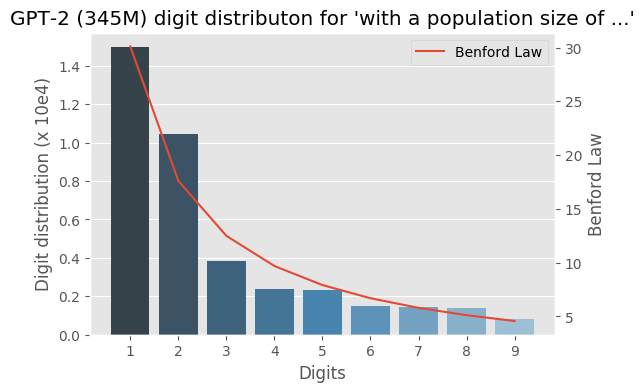
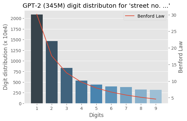
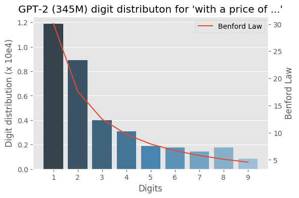
I wrote some months ago about how the Benford law emerges from language models, today I decided to evaluate the same method to check how the GPT-2 would behave with some sentences and it turns out that it seems that it is also capturing these power laws. You can find some plots with the examples below, the plots are showing the probability of the digit given a particular sentence such as “with a population size of”, showing the distribution of: $$P(\{1,2, \ldots, 9\} \vert \text{“with a population size of”})$$ for the GPT-2 medium model (345M):
This website uses cookies to improve your experience. We'll assume you're ok with this, but you can opt-out if you wish. Cookie settingsACCEPT
Privacy & Cookies Policy
Privacy Overview
This website uses cookies to improve your experience while you navigate through the website. Out of these cookies, the cookies that are categorized as necessary are stored on your browser as they are essential for the working of basic functionalities of the website. We also use third-party cookies that help us analyze and understand how you use this website. These cookies will be stored in your browser only with your consent. You also have the option to opt-out of these cookies. But opting out of some of these cookies may have an effect on your browsing experience.
Necessary cookies are absolutely essential for the website to function properly. This category only includes cookies that ensures basic functionalities and security features of the website. These cookies do not store any personal information.
Any cookies that may not be particularly necessary for the website to function and is used specifically to collect user personal data via analytics, ads, other embedded contents are termed as non-necessary cookies. It is mandatory to procure user consent prior to running these cookies on your website.
 Just sharing ~100 slides about PyTorch 2 internals focusing on recent innovations (Dynamo, Inductor, and ExecuTorch). I had a lot of fun preparing this and hope you’ll enjoy it. I’m planning to record it soon.