A small intro on the rationale
So I’m working on a Symbolic Regression Machine written in C/C++ called Shine, which is intended to be a JIT for Genetic Programming libraries (like Pyevolve for instance). The main rationale behind Shine is that we have today a lot of research on speeding Genetic Programming using GPUs (the GPU fever !) or any other special hardware, etc, however we don’t have many papers talking about optimizing GP using the state of art compilers optimizations like we have on clang, gcc, etc.
The “hot spot” or the component that consumes a lot of CPU resources today on Genetic Programming is the evaluation of each individual in order to calculate the fitness of the program tree. This evaluation is often executed on each set of parameters of the “training” set. Suppose you want to make a symbolic regression of a single expression like the Pythagoras Theorem and you have a linear space of parameters from 1.0 to 1000.0 with a step of 0.1 you have 10.000 evaluations for each individual (program tree) of your population !
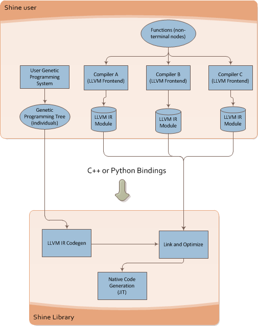
What Shine does is described on the image below:
It takes the individual of the Genetic Programming engine and then converts it to LLVM Intermediate Representation (LLVM assembly language), after that it runs the transformation passes of the LLVM (here is where the true power of modern compilers enter on the GP context) and then the LLVM JIT converts the optimized LLVM IR into native code for the specified target (X86, PowerPC, etc).
You can see below the Shine architecture:
This architecture brings a lot of flexibility for Genetic Programming, you can for instance write functions that could be used later on your individuals on any language supported by the LLVM, what matters to Shine is the LLVM IR, you can use any language that LLVM supports and then use the IR generated by LLVM, you can mix code from C, C++, Ada, Fortran, D, etc and use your functions as non-terminal nodes of your Genetic Programming trees.
Shine is still on its earlier development, it looks a simple idea but I still have a lot of problems to solve, things like how to JIT the evaluation process itself instead of doing calls from Python using ctypes bindings of the JITed trees.
Doing Genetic Programming on the Python AST itself
During the development of Shine, an idea happened to me, that I could use a restricted Python Abstract Syntax Tree (AST) as the representation of individuals on a Genetic Programming engine, the main advantage of this is the flexibility and the possibility to reuse a lot of things. Of course that a shared library written in C/C++ would be useful for a lot of Genetic Programming engines that doesn’t uses Python, but since my spare time to work on this is becoming more and more rare I started to rethink the approach and use Python and the LLVM bindings for LLVM (LLVMPY) and I just discovered that is pretty easy to JIT a restricted set of the Python AST to native code using LLVM, and this is what this post is going to show.
JIT’ing a restricted Python AST
The most amazing part of LLVM is obviously the amount of transformation passes, the JIT and of course the ability to use the entire framework through a simple API (ok, not so simple sometimes). To simplify this example, I’m going to use an arbitrary restricted AST set of the Python AST that supports only subtraction (-), addition (+), multiplication (*) and division (/).
To understand the Python AST, you can use the Python parser that converts source into AST:
>>> import ast
>>> astp = ast.parse("2*7")
>>> ast.dump(astp)
'Module(body=[Expr(value=BinOp(left=Num(n=2), op=Mult(), right=Num(n=7)))])'
What the parse created was an Abstract Syntax Tree containing the BinOp (Binary Operation) with the left operator as the number 2, the right operator as the number 7 and the operation itself as Multiplication(Mult), very easy to understand. What we are going to do to create the LLVM IR is to create a visitor that is going to visit each node of the tree. To do that, we can subclass the Python NodeVisitor class from the ast module. What the NodeVisitor does is to visit each node of the tree and then call the method ‘visit_OPERATOR’ if it exists, when the NodeVisitor is going to visit the node for the BinOp for example, it will call the method ‘visit_BinOp’ passing as parameter the BinOp node itself.
The structure of the class for for the JIT visitor will look like the code below:
# Import the ast and the llvm Python bindings
import ast
from llvm import *
from llvm.core import *
from llvm.ee import *
import llvm.passes as lp

class AstJit(ast.NodeVisitor):
    def __init__(self):
        pass
What we need to do now is to create an initialization method to keep the last state of the JIT visitor, this is needed because we are going to JIT the content of the Python AST into a function and the last instruction of the function needs to return what was the result of the last instruction visited by the JIT. We also need to receive a LLVM Module object in which our function will be created as well the closure type, for the sake of simplicity I’m not type any object, I’m just assuming that all numbers from the expression are integers, so the closure type will be the LLVM integer type.
def __init__(self, module, parameters):
    self.last_state = None
    self.module = module
    # Parameters that will be created on the IR function
    self.parameters = parameters
    self.closure_type = Type.int()
    # An attribute to hold a link to the created function
    # so we can use it to JIT later
    self.func_obj = None
    self._create_builder()


def _create_builder(self):
    # How many parameters of integer type
    params = [self.closure_type] * len(self.parameters)

    # The prototype of the function, returning a integer
    # and receiving the integer parameters
    ty_func = Type.function(self.closure_type, params)

    # Add the function to the module with the name 'func_ast_jit'
    self.func_obj = self.module.add_function(ty_func, 'func_ast_jit')

    # Create an argument in the function for each parameter specified
    for index, pname in enumerate(self.parameters):
        self.func_obj.args[index].name = pname

    # Create a basic block and the builder
    bb = self.func_obj.append_basic_block("entry")
    self.builder = Builder.new(bb)
Now what we need to implement on our visitor is the ‘visit_OPERATOR’ methods for the BinOp and for the Numand Name operators. We will also implement the method to create the return instruction that will return the last state.
# A 'Name' is a node produced in the AST when you
# access a variable, like '2+x+y', 'x' and 'y' are
# the two names created on the AST for the expression.
def visit_Name(self, node):
    # This variable is what function argument ?
    index = self.parameters.index(node.id)
    self.last_state = self.func_obj.args[index]
    return self.last_state

# Here we create a LLVM IR integer constant using the
# Num node, on the expression '2+3' you'll have two
# Num nodes, the Num(n=2) and the Num(n=3).
def visit_Num(self, node):
    self.last_state = Constant.int(self.closure_type, node.n)
    return self.last_state

# The visitor for the binary operation
def visit_BinOp(self, node):
    # Get the operation, left and right arguments
    lhs = self.visit(node.left)
    rhs = self.visit(node.right)
    op = node.op

    # Convert each operation (Sub, Add, Mult, Div) to their
    # LLVM IR integer instruction equivalent
    if isinstance(op, ast.Sub):
        op = self.builder.sub(lhs, rhs, 'sub_t')
    elif isinstance(op, ast.Add):
        op = self.builder.add(lhs, rhs, 'add_t')
    elif isinstance(op, ast.Mult):
        op = self.builder.mul(lhs, rhs, 'mul_t')
    elif isinstance(op, ast.Div):
        op = self.builder.sdiv(lhs, rhs, 'sdiv_t')

    self.last_state = op
    return self.last_state

# Build the return (ret) statement with the last state
def build_return(self):
    self.builder.ret(self.last_state)
And that is it, our visitor is ready to convert a Python AST to a LLVM IR assembly language, to run it we’ll first create a LLVM module and an expression:
module = Module.new('ast_jit_module')
# Note that I'm using two variables 'a' and 'b'
expr = "(2+3*b+33*(10/2)+1+3/3+a)/2"
node = ast.parse(expr)
print ast.dump(node)
Will output:
Module(body=[Expr(value=BinOp(left=BinOp(left=BinOp(left=BinOp(
left=BinOp(left=BinOp(left=Num(n=2), op=Add(), right=BinOp(
left=Num(n=3), op=Mult(), right=Name(id='b', ctx=Load()))), op=Add(),
right=BinOp(left=Num(n=33), op=Mult(), right=Num(n=2))), op=Add(),
right=Num(n=1)), op=Add(), right=Num(n=3)), op=Add(),
right=Name(id='a', ctx=Load())), op=Div(), right=Num(n=2)))])
Now we can finally run our visitor on that generated AST the check the LLVM IR output:
visitor = AstJit(module, ['a', 'b'])
visitor.visit(node)
visitor.build_return()
print module
Will output the LLVM IR:
; ModuleID = 'ast_jit_module'

define i32 @func_ast_jit(i32 %a, i32 %b) {
entry:
  %mul_t = mul i32 3, %b
  %add_t = add i32 2, %mul_t
  %add_t1 = add i32 %add_t, 165
  %add_t2 = add i32 %add_t1, 1
  %add_t3 = add i32 %add_t2, 1
  %add_t4 = add i32 %add_t3, %a
  %sdiv_t = sdiv i32 %add_t4, 2
  ret i32 %sdiv_t
}
Now is when the real fun begins, we want to run LLVM optimization passes to optimize our code with an equivalent GCC -O2 optimization level, to do that we create a PassManagerBuilder and a PassManager, the PassManagerBuilder is the component that adds the passes to the PassManager, you can also manually add arbitrary transformations like dead code elimination, function inlining, etc:
pmb = lp.PassManagerBuilder.new()
# Optimization level
pmb.opt_level = 2

pm = lp.PassManager.new()
pmb.populate(pm)

# Run the passes into the module
pm.run(module)
print module
Will output:
; ModuleID = 'ast_jit_module'

define i32 @func_ast_jit(i32 %a, i32 %b) nounwind readnone {
entry:
  %mul_t = mul i32 %b, 3
  %add_t3 = add i32 %a, 169
  %add_t4 = add i32 %add_t3, %mul_t
  %sdiv_t = sdiv i32 %add_t4, 2
  ret i32 %sdiv_t
}
And here we have the optimized LLVM IR of the Python AST expression. The next step is to JIT that IR into native code and then execute it with some parameters:
ee = ExecutionEngine.new(module)
arg_a = GenericValue.int(Type.int(), 100)
arg_b = GenericValue.int(Type.int(), 42)

retval = ee.run_function(visitor.func_obj, [arg_a, arg_b])
print "Return: %d" % retval.as_int()
Will output:
Return: 197
And that’s it, you have created a AST->LLVM IR converter, optimized the LLVM IR with the transformation passes and then converted it to native code using the LLVM execution engine. I hope you liked =)
* This post is in portuguese
Bom, finalmente chegou meu tão esperado Raspberry Pi, consegui efetuar a compra através de uma fila de espera (estou nesta fila desde o primeiro dia de Março de 2012) na Farnell Newark do Brasil que fez a importação de um (ou mais) lotes da Element 14 e agora está distribuindo aqui no Brasil. Como moro em Porto Alegre no Rio Grande do Sul, o preço total (juntamente com frete) do RPi somaram R$ 182,22 reais, um valor bem acima do esperado para o “computador de $30 dólares”, graças ao nosso gentil governo que como todos já devem ter notado, usa uma EXCELENTE estratégia para incentivar a pesquisa científica, obrigando desta forma os brasileiros a construirem seu próprio hardware usando bambu ou Pau-brasil, mas isto é outra história.
O atendimento da Farnell Newark foi ótimo, a vendedora foi muito atenciosa e sempre respondeu meus questionamentos em um curtíssimo intervalo de tempo, logo após efetuar o pagamento, demorou apenas 1 dia para o aparelho chegar (foi despachado através da UPS). Segue abaixo uma foto dele (clique para ampliar):
Primeiros passos: cartão SD
A primeira tarefa que precisei fazer para fazê-lo funcionar foi a preparação de um cartão SD. Como não consegui encontrar em nenhum lugar que fui um cartão SD de 4GB eu utilizei um micro-SD da Kingston de 4GB (class 4). É importante sempre verificar a Wiki do projeto antes de comprar qualquer cartão SD ou dispositivo USB para o seu Raspberry Pi, pois lá você vai encontrar uma lista de periféricos que comprovadamente funcionam e os que ainda estão problemáticos. Eu aconselho a compra de um cartão class 4 pois houve relatos de problemas com alguns cartões class 10, mas se você já tiver um cartão class 10 não custa tentar a sorte, este é um problema que provavelmente já deve ter sido corrigido no Kernel do Raspbian.
Para preparar o cartão você precisa escolher antes uma distro Linux, eu escolhi o Raspbian que é um port do Debian Wheezy para arm otimizado para “hard float“, o que ajuda bastante na performance de aplicações que fazem bastante uso de operações de ponto flutuante. Além de ser Debian e ter toda a infinidade de pacotes disponíveis no repositório (no momento em que estou escrevendo já existem mais de 30 mil pacotes do Debian já compilados para armhf), ele está funcionando muito bem com todos dispositivos que utilizei até agora (mouse usb, teclado usb, card sd, ethernet, hdmi video/audio, etc.).
Fonte de energia (power supply)
Bom, após ter preparado meu cartão SD eu comprei uma power supply USB, esta da foto abaixo:

Para ligar seu RPi você vai precisar de uma fonte USB de 5V com no mínimo 500mA de corrente disponível, não adianta tentar ligar seu Raspberry Pi na USB do computador.
Como nem tudo é tão simples, ao ligar meu RPi ele logo acustou no boot problemas com o módulo ethernet como este e meu teclado USB não funcionava. O RPi ficava simplesmente travado e sem conexão ethernet alguma, os LEDs nem acendiam.
Sempre desconfie da sua fonte de energia em primeiro lugar ao enfrentar problemas como este, ainda mais aqui no Brasil com todas essas fontes de energia USB “importadas”.
Meu primeiro reflexo foi verificar a voltagem que este power supply estava fornecendo, usando os contatos TP1 e TP2 da placa (você pode ver estes contatos como uns buracos na placa na imagem do RPi). O TP1 está ligado no Vin da fonte de energia e o TP2 no GND (terra) da fonte. Ao ligar o voltímetro, ele mostrou a voltagem abaixo:
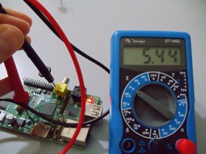
Uma fonte de energia que supostamente deveria fornecer 5v estava fornecendo 5.44V, bem acima do limite de +5% ou -5% tolerado por muitos dispositivos USB como teclados, etc. o RPi possui um regulador de voltagem (SE8117T33) que faz a regulagem da entrada de 5V para 3.3V, este regulador tem o 1.1V como voltagem de dropout, ou seja, para que ele forneça um sinal estável de 3.3V ele precisa ter no mínimo 3.3V+1.1V = 4.4V de entrada, até aí tudo bem, pois estamos fornecendo 5.44V, o problema é que este regulador funciona para distribuição de apenas alguns componentes internos do RPi e não para os dispositivos USB e alguns outros componentes (o Vin da fonte é ligado direto aos periféricos USB), ao fornecer 5.44V ele está ultrapassando um limite de 5% que seria entre 4.75V e 5.25V. Este intervalo de voltagem é o ideal para o seu Raspberry Pi, é sempre importante checar se a sua fonte de energia está dentro deste intervalo e afastado dos limites superiores e inferiores. Um dos fatores que pode causar uma queda da voltagem da sua fonte é o próprio cabo micro USB, que acaba atuando como uma resistência, por isso é sempre bom ter um cabo de qualidade (e curto) e uma fonte de qualidade.
No fim da história tive que trocar minha fonte por uma da Samsung que eu já tinha (do Galaxy Tab P1000-L 7″), este da foto abaixo:

Ao trocar o power supply “importado” por este da Samsung (imagem acima), a voltagem agora ficou:
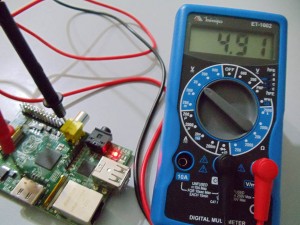
Em estáveis 4.91V, dentro limite aceitável. Após esta troca, tudo passou a funcionar perfeitamente e sem nenhum problema. Fica então a dica para quem for ligar pela primeira vez seu RPi.
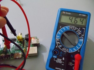
Eu testei também um carregador de iPad da Apple, que ficou também um pouco abaixo do esperado e decidi não usá-lo, segue a foto do carregador e a voltagem dele abaixo:

Finalmente boot !
Após todo este trabalho com o carregador, as coisas finalmente funcionaram corretamente e o RPi fez o boot sem problemas como no screenshot abaixo (estou usando uma TV LG de 42″):
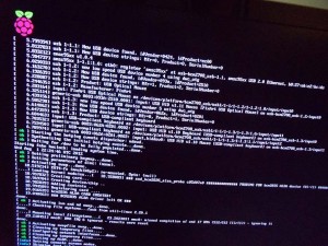
O RPi tem processadores CPU e GPU realmente incríveis, o boot dele é rápido e a saída na TV ficou realmente muito boa em full hd.

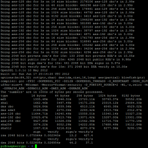
Para testar o processador ARM, que fica em um clock padrão de 700Mhz (você pode fazer overclock até 1Ghz, mas ainda não me aventurei sem um dissipador decente, mas você pode subir para 800Mhz com segurança) eu rodei os benchmarks do OpenSSL, seguem os resultados abaixo:
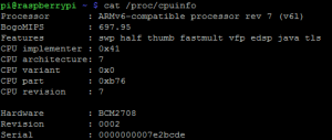
Segue também screenshot do /proc/cpuinfo com os BogoMIPS:
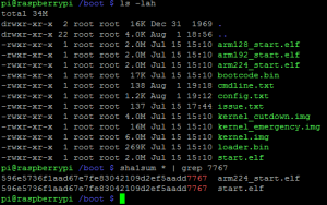
No Raspberry Pi (ao menos usando Raspbian) você pode escolher como será feito o split da memória RAM dele, o padrão vem com 128MB para CPU e 128MB para a GPU (processador gráfico), como eu não estou usando tanto o GPU por hora eu fiz um split de 224MB para o CPU e apenas 32MB para a GPU, para fazer isto você só precisa copiar o arquivo de boot em cima do que é utilizadao para o boot (start.elf) e faz um reboot, segue screenshot dos arquivos abaixo, note que o SHA1 do split de 224 é iguao ao do start.elf:
Após remover 4 dos 6 terminais disponíveis para liberar um pouco mais de memória, a minha memória ficou assim (rodando server do OpenSSH e sem ambiente X):

Fiquei muito satisfeito com este split, você ainda pode fazer outras coisas para liberar memória do seu RPi, como por exemplo trocar o OpenSSH pelo dropbear, etc. Aqui tem um ótimo artigo sobre isto.
Algo que não posso deixar passar também é o Python:

Arduino vs Raspberry Pi
Muitos vêem o Raspberry Pi como um concorrente fatal do Arduino, a percepção que tive porém foi muito diferente. Acredito que o Raspberry Pi vai ser um ótimo companheiro para o Arduino, você inclusive pode utilizar o Arduino na própria USB do Raspberry Pi ou usar alguma outra interface UART ou algo assim. Tenho muitos projetos em mente pra começar usando Arduino e Raspberry Pi, espero poder ter tempo de postar sobre eles aqui no blog. Para quem está ansioso para comparar o tamanho do Raspberry Pi com o Arduino, segue abaixo um comparativo entre o Duemilanove, o RPi e uma moeda de 1 real (não podia faltar hehe):

Conclusão
Você provavelmente não encontrará no Brasil um hardware tão bem elaborado como o Raspberry Pi por estre preço (mesmo alto) de R$ 182,00. Recomendo o RPi para todo mundo que tem o mínimo de interesse, eu poderia ficar aqui falando muita coisa sobre o RPi, sobre os polyfuses usados no design dele, sobre a Gertboard que está por vir, sobre as distribuições disponíveis, etc. Logo farei mais alguns posts sobre os projetos usando o RPi também. Espero que tenham gostado da avaliação.
Review Board is one of these projects that Python community is always proud of, I really think that it became the de facto standard for code reviews nowadays. Review Board comes with an interesting an very useful REST API which you can use to retrieve information about the code reviews, comments, diffs and every single information stored on its database. So, I created a small Python script called rbstats that retrieves information about the Review Requests done by the users and then plots a heat map using matplotlib. I’ll show an example of the use on the Review Board system of the Apache foundation.
To use the tool, just call it with the API URL of the Review Boars system, i.e.:
python rb_stats.py
--max-results 80 https://reviews.apache.org/api
an then you’ll get a graphical plot like this (click to enlarge):
Where the “hottest” points are weighted according to the number of the code reviews that the user have created to the other axis user. You can also plot the statistics by user, for instance of the user benjaminhindman using the autumn colormap and with 400 max results:
python rb_stats.py
--max-results 400
--from-user benjaminhindman
--colormap autumn https://reviews.apache.org/api
Click to enlarge the image:
So, my request to enter on the free and private beta season of the new HP Cloud Services was gently accepted by the HP Cloud team, and today I finally got some time to play with the OpenStack API at HP Cloud. I’ll start with the first impressions I had with the service:
The user interface of the management is very user-friendly, the design is much like of the Twitter Bootstrap, see the screenshot below of the “Compute” page from the “Manage” section:
As you can see, they have a set of 4 Ubuntu images and a CentOS, I think that since they are still in the beta period, soon we’ll have more default images to use.
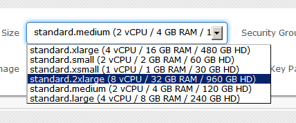
Here is a screenshot of the instance size set:
Since they are using OpenStack, I really think that they should have imported the vocabulary of the OpenStack into the user interface, and instead of calling it “Size”, it would be more sensible to use “Flavour“.
The user interface still doesn’t have many features, something that I would really like to have is a “Stop” or something like that for the instances, only the “Terminate” function is present on the Manage interface, but those are details that they should be still working on since they’re only in beta.
Another important info to cite is that the access to the instances are done through SSH using a generated RSA key that they provide to you.
Let’s dig into the OpenStack API now.
OpenStack API
To access the OpenStack API you’ll need the credentials for the authentication, HP Cloud services provide these keys on the Manage interface for each zone/service you have, see the screenshot below (with keys anonymized of course):
 Now, OpenStack authentication could be done in different schemes, the scheme that I know that HP supports is the token authentication. I know that there is a lot of clients already supporting the OpenStack API (some have no documentation, some have weird API design, etc.), but the aim of this post is to show how easy would be to create a simple interface to access the OpenStack API using Python and Requests (HTTP for Humans !).
Let’s start defining our authentication scheme by sub-classing Requests AuthBase:
[enlighter lang=”python” ]
class OpenStackAuth(AuthBase):
def __init__(self, auth_user, auth_key):
self.auth_key = auth_key
self.auth_user = auth_user
def __call__(self, r):
r.headers[‘X-Auth-User’] = self.auth_user
r.headers[‘X-Auth-Key’] = self.auth_key
return r
[/enlighter]
As you can see, we’re defining the X-Auth-User and the X-Auth-Key in the header of the request with the parameters. These parameters are respectively your Account ID and Access Key we cited earlier. Now, all you have to do is to make the request itself using the authentication scheme, which is pretty easy using Requests:
[enlighter lang=”python”]
ENDPOINT_URL = ‘https://az-1.region-a.geo-1.compute.hpcloudsvc.com/v1.1/’
ACCESS_KEY = ‘Your Access Key’
ACCOUNT_ID = ‘Your Account ID’
response = requests.get(ENDPOINT_URL, auth=OpenStackAuth(ACCOUNT_ID, ACCESS_KEY))
[/enlighter]
And that is it, you’re done with the authentication mechanism using just a few lines of code, and this is how the request is going to be sent to the HP Cloud service server:
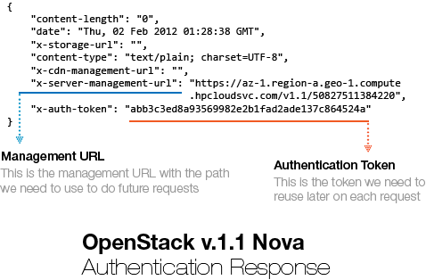
This request is sent to the HP Cloud Endpoint URL (https://az-1.region-a.geo-1.compute.hpcloudsvc.com/v1.1/). Let’s see now how the server answered this authentication request:
You can show this authentication response using Requests by printing the header attribute of the request Response object. You can see that the server answered our request with two important header items: X-Server-Management-URL and the X-Auth-Token. The management URL is now our new endpoint, is the URL we should use to do further requests to the HP Cloud services and the X-Auth-Token is the authentication Token that the server generated based on our credentials, these tokens are usually valid for 24 hours, although I haven’t tested it.
What we need to do now is to sub-class the Requests AuthBase class again but this time defining only the authentication token that we need to use on each new request we’re going to make to the management URL:
[enlighter lang=”python”]
class OpenStackAuthToken(AuthBase):
def __init__(self, request):
self.auth_token = request.headers[‘x-auth-token’]
def __call__(self, r):
r.headers[‘X-Auth-Token’] = self.auth_token
return r
[/enlighter]
Note that the OpenStackAuthToken is receiving now a response request as parameter, copying the X-Auth-Token and setting it on the request.
Let’s consume a service from the OpenStack API v.1.1, I’m going to call the List Servers API function, parse the results using JSON and then show the results on the screen:
[enlighter lang=”python”]
# Get the management URL from the response header
mgmt_url = response.headers[‘x-server-management-url’]
# Create a new request to the management URL using the /servers path
# and the OpenStackAuthToken scheme we created
r_server = requests.get(mgmt_url + ‘/servers’, auth=OpenStackAuthToken(response))
# Parse the response and show it to the screen
json_parse = json.loads(r_server.text)
print json.dumps(json_parse, indent=4)
[/enlighter]
And this is what we get in response to this request:
[enlighter]
{
“servers”: [
{
“id”: 22378,
“uuid”: “e2964d51-fe98-48f3-9428-f3083aa0318e”,
“links”: [
{
“href”: “https://az-1.region-a.geo-1.compute.hpcloudsvc.com/v1.1/20817201684751/servers/22378”,
“rel”: “self”
},
{
“href”: “https://az-1.region-a.geo-1.compute.hpcloudsvc.com/20817201684751/servers/22378”,
“rel”: “bookmark”
}
],
“name”: “Server 22378”
},
{
“id”: 11921,
“uuid”: “312ff473-3d5d-433e-b7ee-e46e4efa0e5e”,
“links”: [
{
“href”: “https://az-1.region-a.geo-1.compute.hpcloudsvc.com/v1.1/20817201684751/servers/11921”,
“rel”: “self”
},
{
“href”: “https://az-1.region-a.geo-1.compute.hpcloudsvc.com/20817201684751/servers/11921”,
“rel”: “bookmark”
}
],
“name”: “Server 11921”
}
]
}
[/enlighter]
And that is it, now you know how to use Requests and Python to consume OpenStack API. If you wish to read more information about the API and how does it works, you can read the documentation here.
– Christian S. Perone
I just tagged and released the v0.2 version of the Stallion. In the change log (Github project page), you can see that a lot of bugs were fixed and some new features were introduced in this release. I added compatibility with almost all Python 2.x versions, PyPy 1.7+ (and probably older versions too), I also fixed the compatibility with the Internet Explorer browser, now you should be able to use Stallion with Chrome, Firefox and IE.
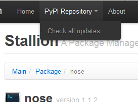
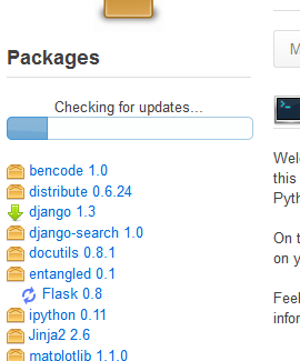
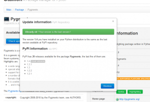
The most important feature introduced is the global checking for updates (a lot of people requested it):
The new checking is under the menu “PyPI Repository”. Another new feature is the refactoring on the visual appearance of the package classifiers:
Some small visual enhancements were also introduced, like the little gray marker next to the selected package:
I hope you liked, I’m looking forward to implement more features as soon as possible, but a new version shouldn’t be released until next year.
Visit the project page at Github to get instructions on how to update or install Stallion.
– Christian S. Perone
I’m happy to announce the first release v.0.1 of the Stallion project. Stallion is a visual Python package manager compatible with Python 2.6 and 2.7 (I still haven’t tested it with Python 2.5).
The motivation behind Stallion is to provide an user friendly visualization with some management features (most of them are still under development) for Python packages installed on your local Python distribution. Stallion is intended to be used specially for Python newcomers.
The project is currently hosted at Github, so feel free to fork, contribute, make suggestion, report bugs, etc.
Installation
All you need to do to install Stallion is to use your favorite Python distribution system, examples:
user@machine:~/$ pip install stallion

or

user@machine:~/$ easy_install stallion
By doing this on your prompt (Windows/Linux), the pip/setuptools will download and install external dependencies (Flask, Jinja, docutils, etc.).
After installing Stallion, you need to start the local server by using:
user@machine:~/$ python -m stallion.main
And if it’s all ok, Stallion will start the server on localhost only at the port 5000, so all you need to do now is to browse into the URL http://localhost:5000
You can also download install packages from the PyPI repository.
See some screenshots (click to enlarge)
Click on the screenshots below to enlarge.
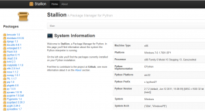
Home
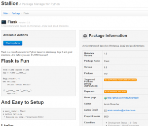
Installed package information
Package metadata
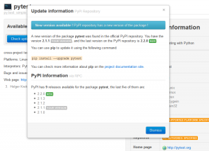
Check PyPI for updates available
PyPI version mismatch diagnosis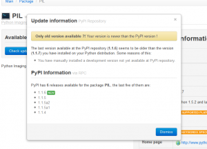
You know, Python represents every object using the low-level C API PyObject (or PyVarObject for variable-size objects) structure, so, concretely, you can cast any Python object pointer to this type; this inheritance is built by hand, every new object must have a leading macro called PyObject_HEAD which defines the PyObject header for the object. The PyObject structure is declared in Include/object.h as:
[enlighter lang=”c”]
typedef struct _object {
PyObject_HEAD
} PyObject;
[/enlighter]
and the PyObject_HEAD macro is defined as:
[enlighter lang=”c”]
#define PyObject_HEAD \
_PyObject_HEAD_EXTRA \
Py_ssize_t ob_refcnt; \
struct _typeobject *ob_type;
[/enlighter]
… with two fields (forget the _PyObject_HEAD_EXTRA, it’s only used for a tracing debug feature) called ob_refcnt and ob_type, representing the reference counting for the object and the type of the object. I know you can use sys.getrefcount to get the reference counting of an object, but hacking the object memory using ctypes is by far more powerful, since you can get the contents of any field of the object (in cases where you don’t have a native API for that), I’ll show more examples later, but lets focus on the reference counting field of the object.
Getting the reference count (ob_refcnt)
So, in Python, we have the built-in function id(), this function returns the identity of the object, but, looking at its definition on CPython implementation, you’ll notice that id() returns the memory address of the object, see the source in Python/bltinmodule.c:
[enlighter lang=”c”]
static PyObject *
builtin_id(PyObject *self, PyObject *v)
{
return PyLong_FromVoidPtr(v);
}
[/enlighter]
… the function PyLong_FromVoidPtr returns a Python long object from a void pointer. So, in CPython, this value is the address of the object in the memory as shown below:
[enlighter lang=”python”]
>>> value = 666
>>> hex(id(value))
‘0x8998e50’ # memory address of the ‘value’ object
[/enlighter]
Now that we have the memory address of the object, we can use the Python ctypes module to get the reference counting by accessing the attribute ob_refcnt, here is the code needed to do that:
[enlighter lang=”python”]
>>> value = 666
>>> value_address = id(value)
>>>
>>> ob_refcnt = ctypes.c_long.from_address(value_address)
>>> ob_refcnt
c_long(1)
[/enlighter]
What I’m doing here is getting the integer value from the ob_refcnt attribute of the PyObject in memory. Let’s add a new reference for the object ‘value’ we created, and then check the reference count again:
[enlighter lang=”python”]
>>> value_ref = value
>>> id(value_ref) == id(value)
True
>>> ob_refcnt
c_long(2)
[/enlighter]
Note that the reference counting was increased by 1 due to the new reference variable called ‘value_ref’.
Interned strings state (ob_sstate)
Now, getting the reference count wasn’t even funny, we already had the sys.getrefcount API for that, but what about the interned state of the strings ? In order to avoid the creation of different allocations for the same string (and to speed comparisons), Python uses a dictionary that works like a “cache” for strings, this dictionary is defined in Objects/stringobject.c:
[enlighter lang=”c”]
/* This dictionary holds all interned strings. Note that references to
strings in this dictionary are *not* counted in the string’s ob_refcnt.
When the interned string reaches a refcnt of 0 the string deallocation
function will delete the reference from this dictionary.
Another way to look at this is that to say that the actual reference
count of a string is: s->ob_refcnt + (s->ob_sstate?2:0)
*/
static PyObject *interned;
[/enlighter]
I also copied here the comment about the dictionary, because is interesting to note that the strings in the dictionary aren’t counted in the string’s ob_refcnt.
So, the interned state of a string object is hold in the attribute ob_sstate of the string object, let’s see the definition of the Python string object:
[enlighter lang=”c”]
typedef struct {
PyObject_VAR_HEAD
long ob_shash;
int ob_sstate;
char ob_sval[1];
/* Invariants:
* ob_sval contains space for ‘ob_size+1’ elements.
* ob_sval[ob_size] == 0.
* ob_shash is the hash of the string or -1 if not computed yet.
* ob_sstate != 0 iff the string object is in stringobject.c’s
* ‘interned’ dictionary; in this case the two references
* from ‘interned’ to this object are *not counted* in ob_refcnt.
*/
} PyStringObject;
[/enlighter]
As you can note, strings objects inherit from the PyObject_VAR_HEAD macro, which defines another header attribute, let’s see the definition to get the complete idea of the structure:
[enlighter lang=”c”]
#define PyObject_VAR_HEAD \
PyObject_HEAD \
Py_ssize_t ob_size; /* Number of items in variable part */
[/enlighter]
The PyObject_VAR_HEAD macro adds another field called ob_size, which is the number of items on the variable part of the Python object (i.e. the number of items on a list object). So, before getting to the ob_sstate field, we need to shift our offset to skip the fields ob_refcnt (long), ob_type (void*) (from PyObject_HEAD), the field ob_size (long) (from PyObject_VAR_HEAD) and the field ob_shash (long) from the PyStringObject. Concretely, we need to skip this offset (3 fields with size long and one field with size void*) of bytes:
[enlighter lang=”python”]
>>> ob_sstate_offset = ctypes.sizeof(ctypes.c_long)*3 + ctypes.sizeof(ctypes.c_voidp)
>>> ob_sstate_offset
16
[/enlighter]
Now, let’s prepare two cases, one that we know that isn’t interned and another that is surely interned, then we’ll force the interned state of the other non-interned string to check the result of the ob_sstate attribute:
[enlighter lang=”python”]
>>> a = “lero”
>>> b = “”.join([“l”, “e”, “r”, “o”])
>>> ctypes.c_long.from_address(id(a) + ob_sstate_offset)
c_long(1)
>>> ctypes.c_long.from_address(id(b) + ob_sstate_offset)
c_long(0)
>>> ctypes.c_long.from_address(id(intern(b)) + ob_sstate_offset)
c_long(1)
[/enlighter]
Note that the interned state for the object “a” is 1 and for the object “b” is 0. After forcing the interned state of the variable “b”, we can see that the field ob_sstate has changed to 1.
Changing internal states (evil mode)
Now, let’s suppose we want to change some internal state of a Python object through the interpreter. Let’s try to change the value of an int object. Int objects are defined in Include/intobject.h:
[enlighter lang=”c”]
typedef struct {
PyObject_HEAD
long ob_ival;
} PyIntObject;
[/enlighter]
As you can see, the internal value of an int is stored in the field ob_ival, to change it, we just need to skip the ob_refcnt (long) and the ob_type (void*) from the PyObject_HEAD:
[enlighter lang=”python”]
>>> value = 666
>>> ob_ival_offset = ctypes.sizeof(ctypes.c_long) + ctypes.sizeof(ctypes.c_voidp)
>>> ob_ival = ctypes.c_int.from_address(id(value)+ob_ival_offset)
>>> ob_ival
c_long(666)
>>> ob_ival.value = 8
>>> value
8
[/enlighter]
And that is it, we have changed the value of the int value directly in the memory.
I hope you liked it, you can play with lots of other Python objects like lists and dicts, note that this method is just intended to show how the Python objects are structured in the memory and how you can change them using the native API, but obviously, you’re not supposed to use this to change the value of ints lol.
Update 11/29/11: you’re not supposed to do such things on your production code or something like that, in this post I’m doing lazy assumptions about arch details like sizes of primitives, etc. Be warned.

