Presentation about an “Achitectural Zoo” of different applications and architectures of CNNs. Presented at Machine Learning Meetup in Porto Alegre yesterday.
The Voynich Manuscript is a hand-written codex written in an unknown system and carbon-dated to the early 15th century (1404–1438). Although the manuscript has been studied by some famous cryptographers of the World War I and II, nobody has deciphered it yet. The manuscript is known to be written in two different languages (Language A and Language B) and it is also known to be written by a group of people. The manuscript itself is always subject of a lot of different hypothesis, including the one that I like the most which is the “culture extinction” hypothesis, supported in 2014 by Stephen Bax. This hypothesis states that the codex isn’t ciphered, it states that the codex was just written in an unknown language that disappeared due to a culture extinction. In 2014, Stephen Bax proposed a provisional, partial decoding of the manuscript, the video of his presentation is very interesting and I really recommend you to watch if you like this codex. There is also a transcription of the manuscript done thanks to the hard-work of many folks working on it since many moons ago.
Word vectors
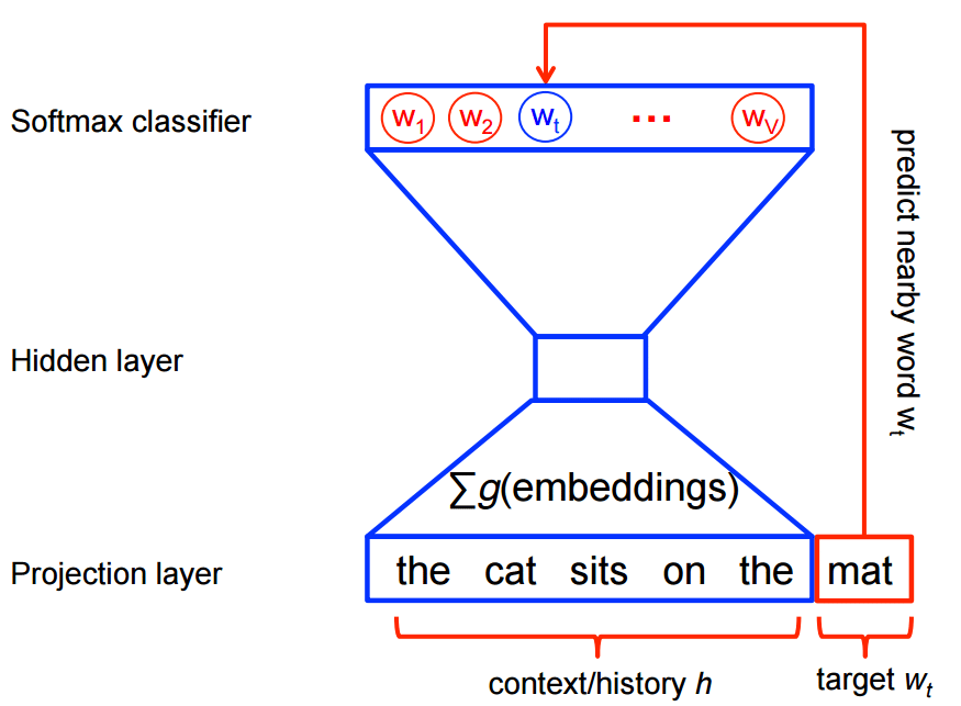
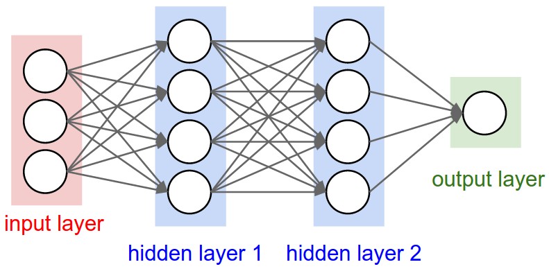
My idea when I heard about the work of Stephen Bax was to try to capture the patterns of the text using word2vec. Word embeddings are created by using a shallow neural network architecture. It is a unsupervised technique that uses supervided learning tasks to learn the linguistic context of the words. Here is a visualization of this architecture from the TensorFlow site:
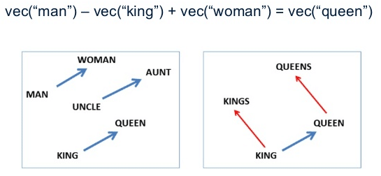
These word vectors, after trained, carry with them a lot of semantic meaning. For instance:
We can see that those vectors can be used in vector operations to extract information about the regularities of the captured linguistic semantics. These vectors also approximates same-meaning words together, allowing similarity queries like in the example below:
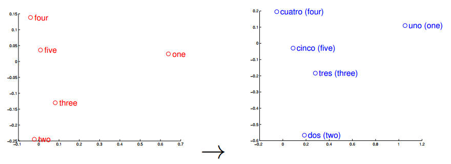
Word vectors can also be used (surprise) for translation, and this is the feature of the word vectors that I think that its most important when used to understand text where we know some of the words translations. I pretend to try to use the words found by Stephen Bax in the future to check if it is possible to capture some transformation that could lead to find similar structures with other languages. A nice visualization of this feature is the one below from the paper “Exploiting Similarities among Languages for Machine Translation“:
This visualization was made using gradient descent to optimize a linear transformation between the source and destination language word vectors. As you can see, the structure in Spanish is really close to the structure in English.
EVA Transcription
To train this model, I had to parse and extract the transcription from the EVA (European Voynich Alphabet) to be able to feed the Voynich sentences into the word2vec model. This EVA transcription has the following format:
The first data between “<” and “>” has information about the folio (page), line and author of the transcription. The transcription block above is the transcription for the first two lines of the first folio of the manuscript below:
Part of the “f1r”
As you can see, the EVA contains some code characters, like for instance “!”, “*” and they all have some meaning, like to inform that the author doing that translation is not sure about the character in that position, etc. EVA also contains transcription from different authors for the same line of the folio.
To convert this transcription to sentences I used only lines where the authors were sure about the entire line and I used the first line where the line satisfied this condition. I also did some cleaning on the transcription to remove the drawings names from the text, like: “text.text.text-{plant}text” -> “text text texttext”.
After this conversion from the EVA transcript to sentences compatible with the word2vec model, I trained the model to provide 100-dimensional word vectors for the words of the manuscript.
Vector space visualizations using t-SNE
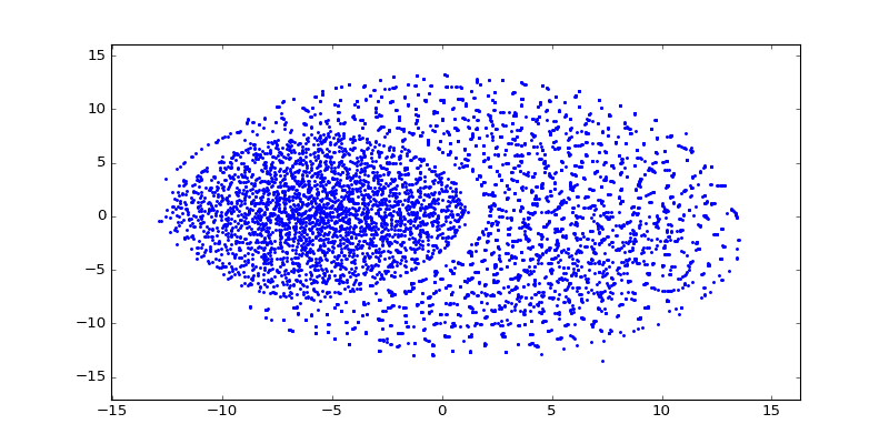
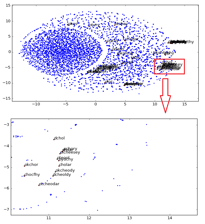
After training word vectors, I created a visualization of the 100-dimensional vectors into a 2D embedding space using t-SNE algorithm:
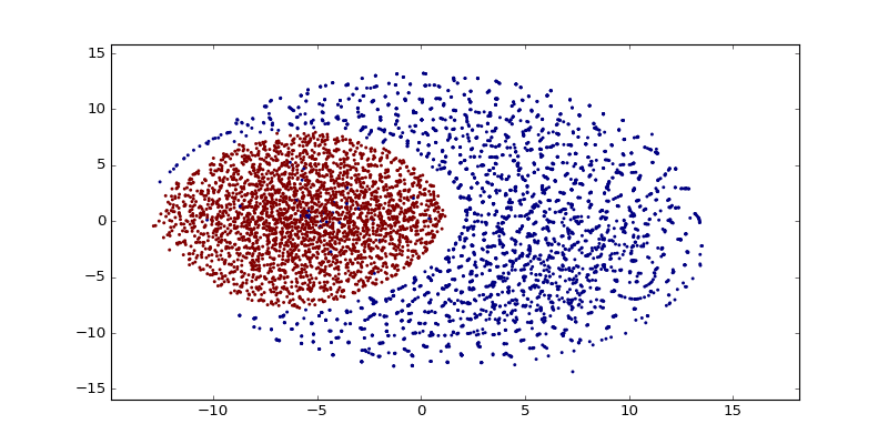
As you can see there are a lot of small clusters and there visually two big clusters, probably accounting for the two different languages used in the Codex (I still need to confirm this regarding the two languages aspect). After clustering it with DBSCAN (using the original word vectors, not the t-SNE transformed vectors), we can clearly see the two major clusters:
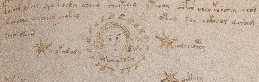
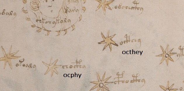
Now comes the really interesting and useful part of the word vectors, if use a star name from the folio below (it’s pretty obvious why it is know that this is probably a star name):
I get really interesting similar words, like for instance the ocphy and other close star names:
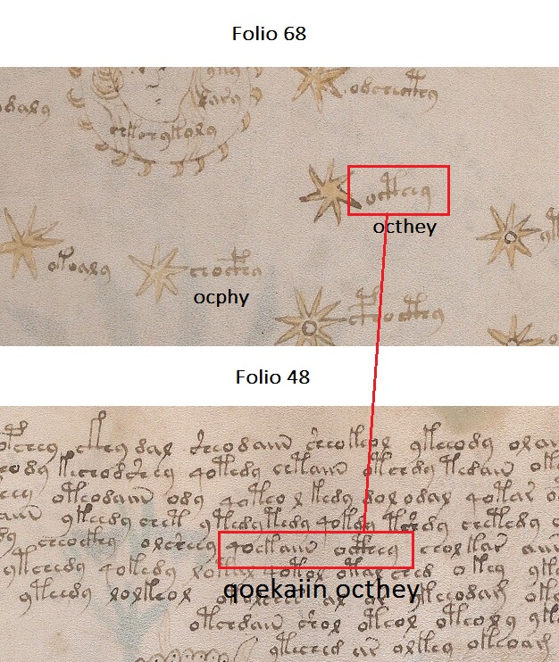
It also returns the word “qoekaiin” from the folio 48, that precedes the same star name:
As you can see, word vectors are really useful to find some linguistic structures, we can also create another plot, showing how close are the star names in the 2D embedding space visualization created using t-SNE:
As you can see, we zoomed the major cluster of stars and we can see that they are really all grouped together in the vector space. These representations can be used for instance to infer plat names from the herbal section, etc.
My idea was to show how useful word vectors are to analyze unknown codex texts, I hope you liked and I hope that this could be somehow useful for other people how are also interested in this amazing manuscript.
If you are following some Machine Learning news, you certainly saw the work done by Ryan Dahl on Automatic Colorization (Hacker News comments, Reddit comments). This amazing work uses pixel hypercolumn information extracted from the VGG-16 network in order to colorize images. Samim also used the network to process Black & White video frames and produced the amazing video below:
Colorizing Black&White Movies with Neural Networks (video by Samim, network by Ryan)
But how does this hypercolumns works ? How to extract them to use on such variety of pixel classification problems ? The main idea of this post is to use the VGG-16 pre-trained network together with Keras and Scikit-Learn in order to extract the pixel hypercolumns and take a superficial look at the information present on it. I’m writing this because I haven’t found anything in Python to do that and this may be really useful for others working on pixel classification, segmentation, etc.
Hypercolumns
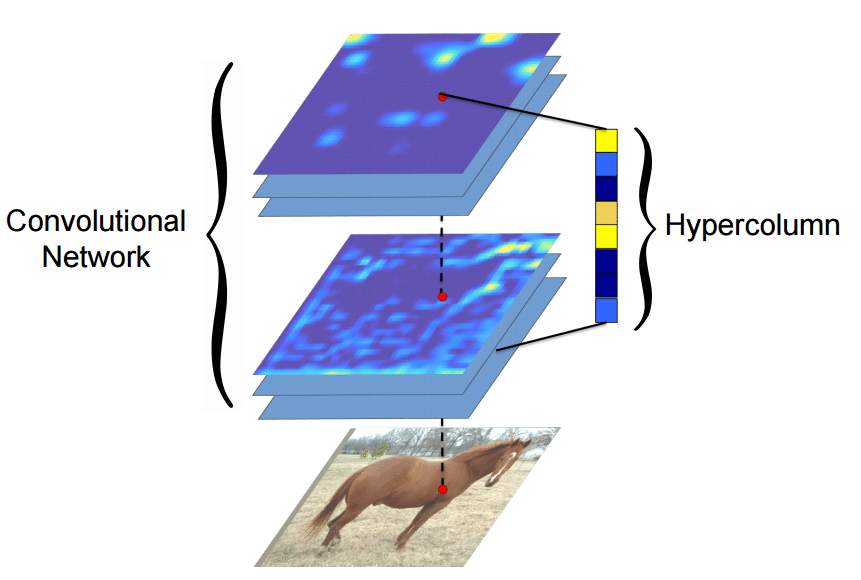
Many algorithms using features from CNNs (Convolutional Neural Networks) usually use the last FC (fully-connected) layer features in order to extract information about certain input. However, the information in the last FC layer may be too coarse spatially to allow precise localization (due to sequences of maxpooling, etc.), on the other side, the first layers may be spatially precise but will lack semantic information. To get the best of both worlds, the authors of the hypercolumn paper define the hypercolumn of a pixel as the vector of activations of all CNN units “above” that pixel.
Hypercolumn Extraction (by Hypercolumns for Object Segmentation and Fine-grained Localization)
The first step on the extraction of the hypercolumns is to feed the image into the CNN (Convolutional Neural Network) and extract the feature map activations for each location of the image. The tricky part is when the feature maps are smaller than the input image, for instance after a pooling operation, the authors of the paper then do a bilinear upsampling of the feature map in order to keep the feature maps on the same size of the input. There are also the issue with the FC (fully-connected) layers, because you can’t isolate units semantically tied only to one pixel of the image, so the FC activations are seen as 1×1 feature maps, which means that all locations shares the same information regarding the FC part of the hypercolumn. All these activations are then concatenated to create the hypercolumn. For instance, if we take the VGG-16 architecture to use only the first 2 convolutional layers after the max pooling operations, we will have a hypercolumn with the size of:
64 filters (first conv layer before pooling)
+
128 filters (second conv layer before pooling ) = 192 features
This means that each pixel of the image will have a 192-dimension hypercolumn vector. This hypercolumn is really interesting because it will contain information about the first layers (where we have a lot of spatial information but little semantic) and also information about the final layers (with little spatial information and lots of semantics). Thus this hypercolumn will certainly help in a lot of pixel classification tasks such as the one mentioned earlier of automatic colorization, because each location hypercolumn carries the information about what this pixel semantically and spatially represents. This is also very helpful on segmentation tasks (you can see more about that on the original paper introducing the hypercolumn concept).
Everything sounds cool, but how do we extract hypercolumns in practice ?
VGG-16
Before being able to extract the hypercolumns, we’ll setup the VGG-16 pre-trained network, because you know, the price of a good GPU (I can’t even imagine many of them) here in Brazil is very expensive and I don’t want to sell my kidney to buy a GPU.
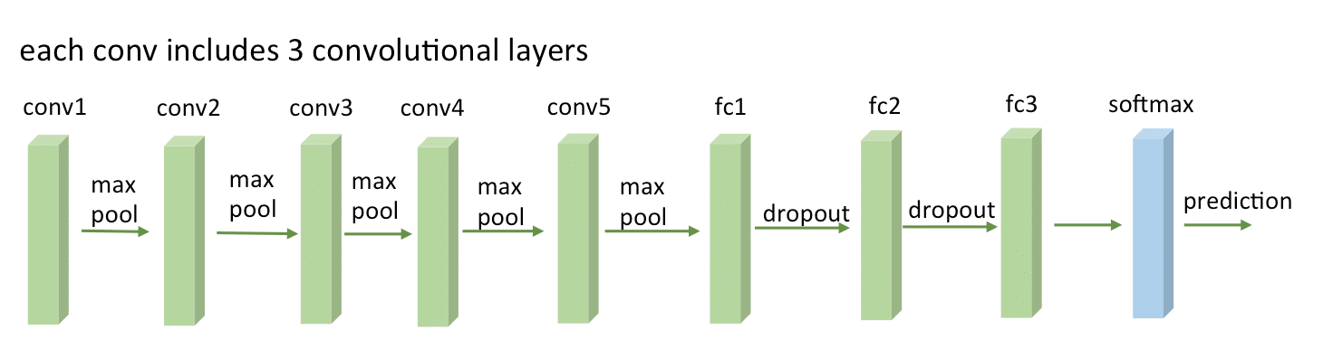
VGG16 Network Architecture (by Zhicheng Yan et al.)
To setup a pretrained VGG-16 network on Keras, you’ll need to download the weights file from here (vgg16_weights.h5 file with approximately 500MB) and then setup the architecture and load the downloaded weights using Keras (more information about the weights file and architecture here):
from matplotlib import pyplot as plt

import theano
import cv2
import numpy as np
import scipy as sp

from keras.models import Sequential
from keras.layers.core import Flatten, Dense, Dropout
from keras.layers.convolutional import Convolution2D, MaxPooling2D
from keras.layers.convolutional import ZeroPadding2D
from keras.optimizers import SGD

from sklearn.manifold import TSNE
from sklearn import manifold
from sklearn import cluster
from sklearn.preprocessing import StandardScaler

def VGG_16(weights_path=None):
    model = Sequential()
    model.add(ZeroPadding2D((1,1),input_shape=(3,224,224)))
    model.add(Convolution2D(64, 3, 3, activation='relu'))
    model.add(ZeroPadding2D((1,1)))
    model.add(Convolution2D(64, 3, 3, activation='relu'))
    model.add(MaxPooling2D((2,2), stride=(2,2)))

    model.add(ZeroPadding2D((1,1)))
    model.add(Convolution2D(128, 3, 3, activation='relu'))
    model.add(ZeroPadding2D((1,1)))
    model.add(Convolution2D(128, 3, 3, activation='relu'))
    model.add(MaxPooling2D((2,2), stride=(2,2)))

    model.add(ZeroPadding2D((1,1)))
    model.add(Convolution2D(256, 3, 3, activation='relu'))
    model.add(ZeroPadding2D((1,1)))
    model.add(Convolution2D(256, 3, 3, activation='relu'))
    model.add(ZeroPadding2D((1,1)))
    model.add(Convolution2D(256, 3, 3, activation='relu'))
    model.add(MaxPooling2D((2,2), stride=(2,2)))

    model.add(ZeroPadding2D((1,1)))
    model.add(Convolution2D(512, 3, 3, activation='relu'))
    model.add(ZeroPadding2D((1,1)))
    model.add(Convolution2D(512, 3, 3, activation='relu'))
    model.add(ZeroPadding2D((1,1)))
    model.add(Convolution2D(512, 3, 3, activation='relu'))
    model.add(MaxPooling2D((2,2), stride=(2,2)))

    model.add(Flatten())
    model.add(Dense(4096, activation='relu'))
    model.add(Dropout(0.5))
    model.add(Dense(4096, activation='relu'))
    model.add(Dropout(0.5))
    model.add(Dense(1000, activation='softmax'))

    if weights_path:
        model.load_weights(weights_path)

    return model
As you can see, this is a very simple code to declare the VGG16 architecture and load the pre-trained weights (together with Python imports for the required packages). After that we’ll compile the Keras model:
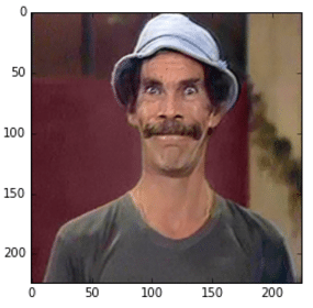
im_original = cv2.resize(cv2.imread('madruga.jpg'), (224, 224))
im = im_original.transpose((2,0,1))
im = np.expand_dims(im, axis=0)
im_converted = cv2.cvtColor(im_original, cv2.COLOR_BGR2RGB)
plt.imshow(im_converted)
Image used
As we can see, we loaded the image, fixed the axes and then we can now feed the image into the VGG-16 to get the predictions:
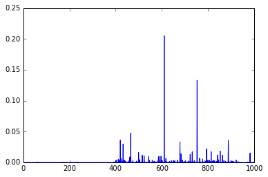
out = model.predict(im)
plt.plot(out.ravel())
Predictions
As you can see, these are the final activations of the softmax layer, the class with the “jersey, T-shirt, tee shirt” category.
Extracting arbitrary feature maps
Now, to extract the feature map activations, we’ll have to being able to extract feature maps from arbitrary convolutional layers of the network. We can do that by compiling a Theano function using the get_output() method of Keras, like in the example below:
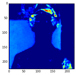
In the example above, I’m compiling a Theano function to get the 3 layer (a convolutional layer) feature map and then showing only the 3rd feature map. Here we can see the intensity of the activations. If we get feature maps of the activations from the final layers, we can see that the extracted features are more abstract, like eyes, etc. Look at this example below from the 15th convolutional layer:
As you can see, this second feature map is extracting more abstract features. And you can also note that the image seems to be more stretched when compared with the feature we saw earlier, that is because the the first feature maps has 224×224 size and this one has 56×56 due to the downscaling operations of the layers before the convolutional layer, and that is why we lose a lot of spatial information.
Extracting hypercolumns
Now finally let’s extract the hypercolumns of arbitrary set of layers. To do that, we will define a function to extract these hypercolumns:
def extract_hypercolumn(model, layer_indexes, instance):
    layers = [model.layers[li].get_output(train=False) for li in layer_indexes]
    get_feature = theano.function([model.layers[0].input], layers,
                                  allow_input_downcast=False)
    feature_maps = get_feature(instance)
    hypercolumns = []
    for convmap in feature_maps:
        for fmap in convmap[0]:
            upscaled = sp.misc.imresize(fmap, size=(224, 224),
                                        mode="F", interp='bilinear')
            hypercolumns.append(upscaled)

    return np.asarray(hypercolumns)
As we can see, this function will expect three parameters: the model itself, an list of layer indexes that will be used to extract the hypercolumn features and an image instance that will be used to extract the hypercolumns. Let’s now test the hypercolumn extraction for the first 2 convolutional layers:
layers_extract = [3, 8]
hc = extract_hypercolumn(model, layers_extract, im)
That’s it, we extracted the hypercolumn vectors for each pixel. The shape of this “hc” variable is: (192L, 224L, 224L), which means that we have a 192-dimensional hypercolumn for each one of the 224×224 pixel (a total of 50176 pixels with 192 hypercolumn feature each).
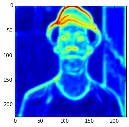
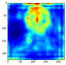
Let’s plot the average of the hypercolumns activations for each pixel:
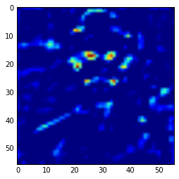
Ad you can see, those first hypercolumn activations are all looking like edge detectors, let’s see how these hypercolumns looks like for the layers 22 and 29:
As we can see now, the features are really more abstract and semantically interesting but with spatial information a little fuzzy.
Remember that you can extract the hypercolumns using all the initial layers and also the final layers, including the FC layers. Here I’m extracting them separately to show how they differ in the visualization plots.
Simple hypercolumn pixel clustering
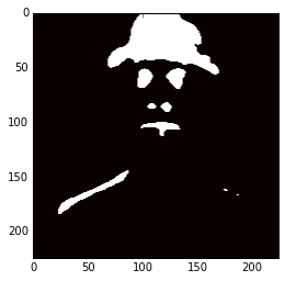
Now, you can do a lot of things, you can use these hypercolumns to classify pixels for some task, to do automatic pixel colorization, segmentation, etc. What I’m going to do here just as an experiment, is to use the hypercolumns (from the VGG-16 layers 3, 8, 15, 22, 29) and then cluster it using KMeans with 2 clusters:
Now you can imagine how useful hypercolumns can be to tasks like keypoints extraction, segmentation, etc. It’s a very elegant, simple and useful concept.
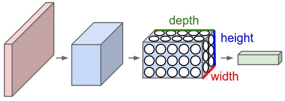
Convolutional neural networks (or ConvNets) are biologically-inspired variants of MLPs, they have different kinds of layers and each different layer works different than the usual MLP layers. If you are interested in learning more about ConvNets, a good course is the CS231n – Convolutional Neural Newtorks for Visual Recognition. The architecture of the CNNs are shown in the images below:
As you can see, the ConvNets works with 3D volumes and transformations of these 3D volumes. I won’t repeat in this post the entire CS231n tutorial, so if you’re really interested, please take time to read before continuing.
Lasagne and nolearn
One of the Python packages for deep learning that I really like to work with is Lasagne and nolearn. Lasagne is based on Theano so the GPU speedups will really make a great difference, and their declarative approach for the neural networks creation are really helpful. The nolearn libary is a collection of utilities around neural networks packages (including Lasagne) that can help us a lot during the creation of the neural network architecture, inspection of the layers, etc.
What I’m going to show in this post, is how to build a simple ConvNet architecture with some convolutional and pooling layers. I’m also going to show how you can use a ConvNet to train a feature extractor and then use it to extract features before feeding them into different models like SVM, Logistic Regression, etc. Many people use pre-trained ConvNet models and then remove the last output layer to extract the features from ConvNets that were trained on ImageNet datasets. This is usually called transfer learning because you can use layers from other ConvNets as feature extractors for different problems, since the first layer filters of the ConvNets works as edge detectors, they can be used as general feature detectors for other problems.
Loading the MNIST dataset
The MNIST dataset is one of the most traditional datasets for digits classification. We will use a pickled version of it for Python, but first, lets import the packages that we will need to use:
import matplotlib
import matplotlib.pyplot as plt
import matplotlib.cm as cm

from urllib import urlretrieve
import cPickle as pickle
import os
import gzip

import numpy as np
import theano

import lasagne
from lasagne import layers
from lasagne.updates import nesterov_momentum

from nolearn.lasagne import NeuralNet
from nolearn.lasagne import visualize

from sklearn.metrics import classification_report
from sklearn.metrics import confusion_matrix
As you can see, we are importing matplotlib for plotting some images, some native Python modules to download the MNIST dataset, numpy, theano, lasagne, nolearn and some scikit-learn functions for model evaluation.
After that, we define our MNIST loading function (this is pretty the same function used in the Lasagne tutorial):
As you can see, we are downloading the MNIST pickled dataset and then unpacking it into the three different datasets: train, validation and test. After that we reshape the image contents to prepare them to input into the Lasagne input layer later and we also convert the numpy array types to uint8 due to the GPU/theano datatype restrictions.
After that, we’re ready to load the MNIST dataset and inspect it:
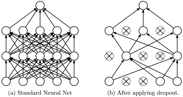
As you can see, in the parameter layers we’re defining a dictionary of tuples with the layer names/types and then we define the parameters for these layers. Our architecture here is using two convolutional layers with poolings and then a fully connected layer (dense layer) and the output layer. There are also dropouts between some layers, the dropout layer is a regularizer that randomly sets input values to zero to avoid overfitting (see the image below).
Dropout layer effect (from CS231n website).
After calling the train method, the nolearn package will show status of the learning process, in my machine with my humble GPU I got the results below:
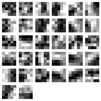
The code above will plot the following filters below:
The first layer 5x5x32 filters.
As you can see, the nolearn plot_conv_weights plots all the filters present in the layer we specified.
Theano layer functions and Feature Extraction
Now it is time to create theano-compiled functions that will feed-forward the input data into the architecture up to the layer you’re interested. I’m going to get the functions for the output layer and also for the dense layer before the output layer:
As you can see, we have now two theano functions called f_output and f_dense (for the output and dense layers). Please note that in order to get the layers here we are using a extra parameter called “deterministic“, this is to avoid the dropout layers affecting our feed-forward pass.
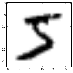
We can now convert an example instance to the input format and then feed it into the theano function for the output layer:
instance = X_test[0][None, :, :]
%timeit -n 500 f_output(instance)

500 loops, best of 3: 858 µs per loop
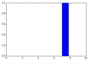
As you can see, the f_output function takes an average of 858 µs. We can also plot the output layer activations for the instance:
pred = f_output(instance)
N = pred.shape[1]
plt.bar(range(N), pred.ravel())
The code above will create the following plot:
Output layer activations.
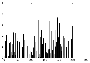
As you can see, the digit was recognized as the digit 7. The fact that you can create theano functions for any layer of the network is very useful because you can create a function (like we did before) to get the activations for the dense layer (the one before the output layer) and you can use these activations as features and use your neural network not as classifier but as a feature extractor. Let’s plot now the 256 unit activations for the dense layer:
pred = f_dense(instance)
N = pred.shape[1]
plt.bar(range(N), pred.ravel())
The code above will create the following plot below:
Dense layer activations.
You can now use the output of the these 256 activations as features on a linear classifier like Logistic Regression or SVM.
Update – 05 Dec 2017: Google just announced that it will be commited to the development of a new released version of the S2 library, amazing news, repository can be found here.
Google’s S2 library is a real treasure, not only due to its capabilities for spatial indexing but also because it is a library that was released more than 4 years ago and it didn’t get the attention it deserved. The S2 library is used by Google itself on Google Maps, MongoDB engine and also by Foursquare, but you’re not going to find any documentation or articles about the library anywhere except for a paper by Foursquare, a Google presentation and the source code comments. You’ll also struggle to find bindings for the library, the official repository has missing Swig files for the Python library and thanks to some forks we can have a partial binding for the Python language (I’m going to it use for this post). I heard that Google is actively working on the library right now and we are probably soon going to get more details about it when they release this work, but I decided to share some examples about the library and the reasons why I think that this library is so cool.
The way to the cells
You’ll see this “cell” concept all around the S2 code. The cells are an hierarchical decomposition of the sphere (the Earth on our case, but you’re not limited to it) into compact representations of regions or points. Regions can also be approximated using these same cells, that have some nice features:
They are compact (represented by 64-bit integers)
They have resolution for geographical features
They are hierarchical (thay have levels, and similar levels have similar areas)
The containment query for arbitrary regions are really fast
The S2 library starts by projecting the points/regions of the sphere into a cube, and each face of the cube has a quad-tree where the sphere point is projected into. After that, some transformation occurs (for more details on why, see the Google presentation) and the space is discretized, after that the cells are enumerated on a Hilbert Curve, and this is why this library is so nice, the Hilbert curve is a space-filling curve that converts multiple dimensions into one dimension that has an special spatial feature: it preserves the locality.
Hilbert Curve
Hilbert Curve
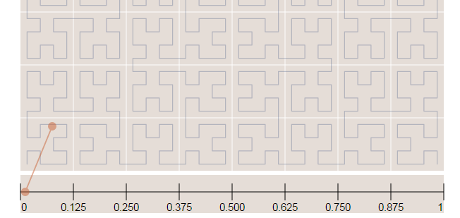
The Hilbert curve is space-filling curve, which means that its range covers the entire n-dimensional space. To understand how this works, you can imagine a long string that is arranged on the space in a special way such that the string passes through each square of the space, thus filling the entire space. To convert a 2D point along to the Hilbert curve, you just need select the point on the string where the point is located. An easy way to understand it is to use this iterative example where you can click on any point of the curve and it will show where in the string the point is located and vice-versa.
In the image below, the point in the very beggining of the Hilbert curve (the string) is located also in the very beginning along curve (the curve is represented by a long string in the bottom of the image):
Hilbert Curve
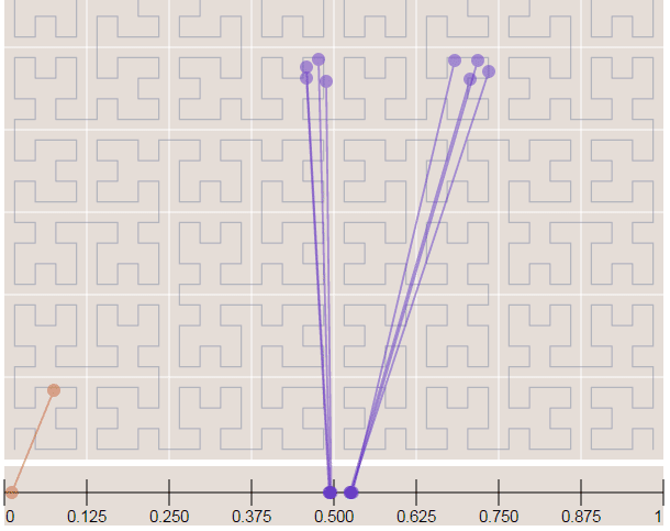
Now in the image below where we have more points, it is easy to see how the Hilbert curve is preserving the spatial locality. You can note that points closer to each other in the curve (in the 1D representation, the line in the bottom) are also closer in the 2D dimensional space (in the x,y plane). However, note that the opposite isn’t quite true because you can have 2D points that are close to each other in the x,y plane that aren’t close in the Hilbert curve.
Hilbert Curve
Since S2 uses the Hilbert Curve to enumerate the cells, this means that cell values close in value are also spatially close to each other. When this idea is combined with the hierarchical decomposition, you have a very fast framework for indexing and for query operations. Before we start with the pratical examples, let’s see how the cells are represented in 64-bit integers.
If you are interested in Hilbert Curves, I really recommend this article, it is very intuitive and show some properties of the curve.
The cell representation
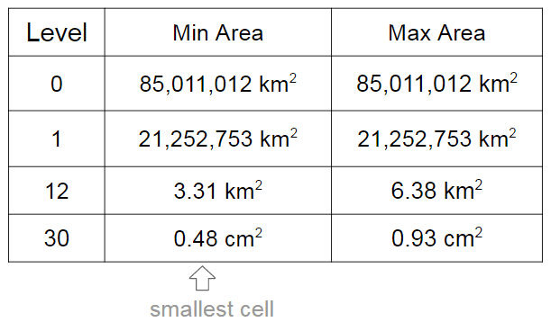
As I already mentioned, the cells have different levels and different regions that they can cover. In the S2 library you’ll find 30 levels of hierachical decomposition. The cell level and the area range that they can cover is shown in the Google presentation in the slide that I’m reproducing below:
Cell areas
As you can see, a very cool result of the S2 geometry is that every cm² of the earth can be represented using a 64-bit integer.
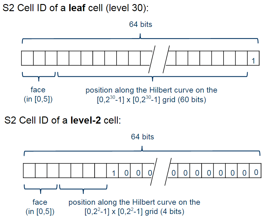
The cells are represented using the following schema:
Cell Representation Schema (images from the original Google presentation)
The first one is representing a leaf cell, a cell with the minimum area usually used to represent points. As you can see, the 3 initial bits are reserved to store the face of the cube where the point of the sphere was projected, then it is followed by the position of the cell in the Hilbert curve always followed by a “1” bit that is a marker that will identify the level of the cell.
So, to check the level of the cell, all that is required is to check where the last “1” bit is located in the cell representation. The checking of containment, to verify if a cell is contained in another cell, all you just have to do is to do a prefix comparison. These operations are really fast and they are possible only due to the Hilbert Curve enumeration and the hierarchical decomposition method used.
Covering regions
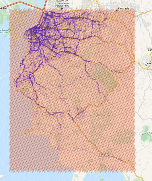
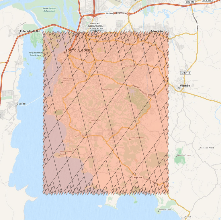
So, if you want to generate cells to cover a region, you can use a method of the library where you specify the maximum number of the cells, the maximum cell level and the minimum cell level to be used and an algorithm will then approximate this region using the specified parameters. In the example below, I’m using the S2 library to extract some Machine Learning binary features using level 15 cells:
Cells at level 15 – binary features for Machine Learning
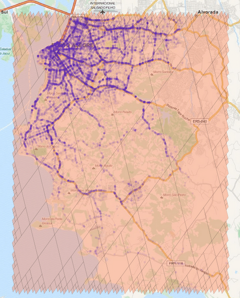
The cells regions are here represented in the image above using transparent polygons over the entire region of interest of my city. Since I used the level 15 both for minimum and maximum level, the cells are all covering similar region areas. If I change the minimum level to 8 (thus allowing the possibility of using larger cells), the algorithm will approximate the region in a way that it will provide the smaller number of cells and also trying to keep the approximation precise like in the example below:
Covering using range from 8 to 15 (levels)
As you can see, we have now a covering using larger cells in the center and to cope with the borders we have an approximation using smaller cells (also note the quad-trees).
Examples
* In this tutorial I used the Python 2.7 bindings from the following repository. The instructions to compile and install it are present in the readme of the repository so I won’t repeat it here.
The first step to convert Latitude/Longitude points to the cell representation are shown below:
As you can see, we first create an object of the class S2LatLng to represent the lat/lng point and then we feed it into the S2CellId class to build the cell representation. After that, we can get the level and id of the class. There is also a method called ToToken that converts the integer representation to a compact alphanumerical representation that you can parse it later using FromToken method.
You can also get the parent cell of that cell (one level above it) and use containment methods to check if a cell is contained by another cell:
As you can see, the level of the parent is one above the children cell (in our case, a leaf cell). The ids are also very similar except for the level of the cell and the containment checking is really fast (it is only checking the range of the children cells of the parent cell).
These cells can be stored on a database and they will perform quite well on a BTree index. In order to create a collection of cells that will cover a region, you can use the S2RegionCoverer class like in the example below:
First of all, we defined a S2LatLngRect which is a rectangle delimiting the region that we want to cover. There are also other classes that you can use (to build polygons for instance), the S2RegionCoverer works with classes that uses the S2Region class as base class. After defining the rectangle, we instantiate the S2RegionCoverer and then set the aforementioned min/max levels and the max number of the cells that we want the approximation to generate.
If you wish to plot the covering, you can use Cartopy, Shapely and matplotlib, like in the example below:
import matplotlib.pyplot as plt

from s2 import *

from shapely.geometry import Polygon

import cartopy.crs as ccrs
import cartopy.io.img_tiles as cimgt

proj = cimgt.MapQuestOSM()
plt.figure(figsize=(20,20), dpi=200)
ax = plt.axes(projection=proj.crs)

ax.add_image(proj, 12)
ax.set_extent([-51.411886, -50.922470,
               -30.301314, -29.94364])

region_rect = S2LatLngRect(
    S2LatLng.FromDegrees(-51.264871, -30.241701),
    S2LatLng.FromDegrees(-51.04618, -30.000003))

coverer = S2RegionCoverer()
coverer.set_min_level(8)
coverer.set_max_level(15)
coverer.set_max_cells(500)
covering = coverer.GetCovering(region_rect)

geoms = []
for cellid in covering:
    new_cell = S2Cell(cellid)
    vertices = []
    for i in xrange(0, 4):
        vertex = new_cell.GetVertex(i)
        latlng = S2LatLng(vertex)
        vertices.append((latlng.lat().degrees(),
                         latlng.lng().degrees()))

    geo = Polygon(vertices)
    geoms.append(geo)

print "Total Geometries: {}".format(len(geoms))

ax.add_geometries(geoms, ccrs.PlateCarree(), facecolor='coral',
                  edgecolor='black', alpha=0.4)
plt.show()
And the result will be the one below:
The covering cells.
There are a lot of stuff in the S2 API, and I really recommend you to explore and read the source-code, it is really helpful. The S2 cells can be used for indexing and in key-value databases, it can be used on B Trees with really good efficiency and also even for Machine Learning purposes (which is my case), anyway, it is a very useful tool that you should keep in your toolbox. I hope you enjoyed this little tutorial !
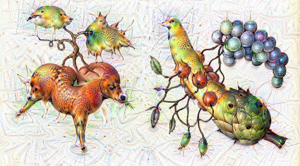
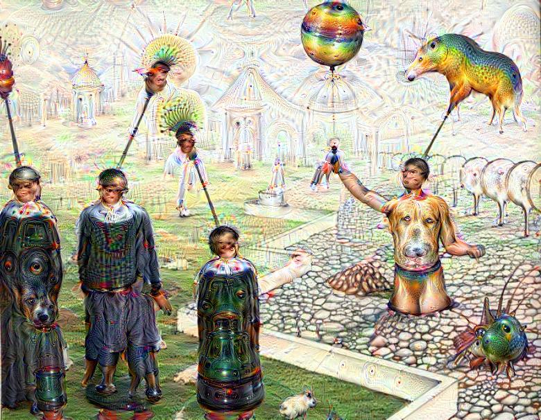
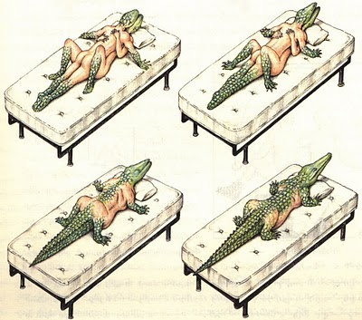
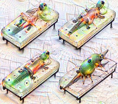
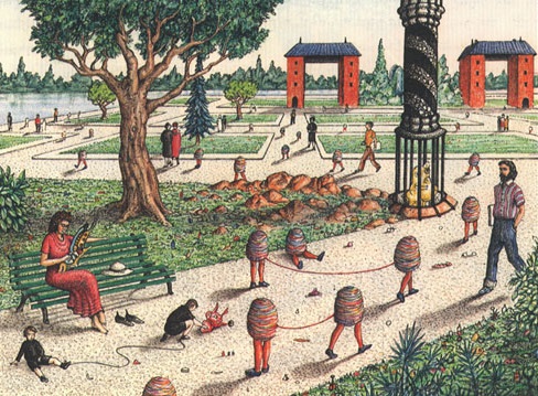
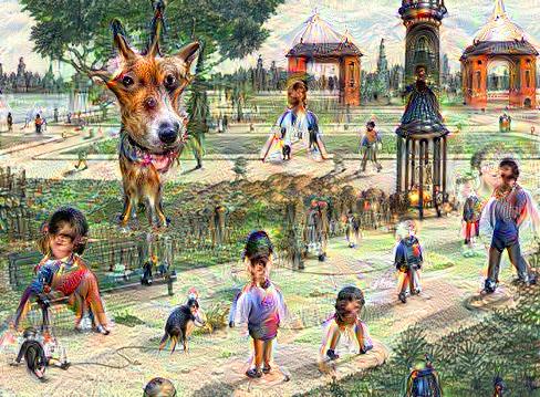
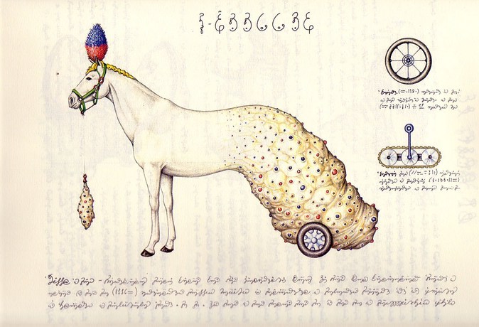
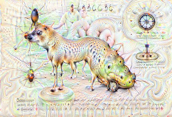
Some time ago I received the Luigi’s Codex Seraphinianus book, for those who still didn’t had a chance to take a look, I really recommend you to buy the book, this is the kind of book that will certainly leave a weirdness in your senses. Codex looks like a treatise of a obscure world, and the Codex alone is by far the most weirdest book I’ve ever seen, so I decided to use the GoogleNet model to create the inceptionisms (using the code based on Caffe, that Google kindly released) with some selected images from the Codex. The result of this process created some very interesting images that I decided to share below (click to enlarge):
Original Codex Seraphinianus image.Deep dreams.The original Codex Seraphinianus image.Deep dreams.The original Codex Seraphinianus image.Deep dreams.The original Codex Seraphinianus image.Deep dreams.The original Codex Seraphinianus image.Deep Dreams
After flying this past weekend (together with Gabriel and Leandro) with Gabriel’s drone (which is an handmade APM 2.6 based quadcopter) in our town (Porto Alegre, Brasil), I decided to implement a tracking for objects using OpenCV and Python and check how the results would be using simple and fast methods like Meanshift. The result was very impressive and I believe that there is plenty of room for optimization, but the algorithm is now able to run in real time using Python with good results and with a Full HD resolution of 1920×1080 and 30 fps.
Here is the video of the flight that was piloted by Gabriel:
See it in Full HD for more details.
The algorithm can be described as follows and it is very simple (less than 50 lines of Python) and straightforward:
A ROI (Region of Interest) is defined, in this case the building that I want to track
The normalized histogram and back-projection are calculated
The Meanshift algorithm is used to track the ROI
The entire code for the tracking is described below:
import numpy as np
import cv2

def run_main():
    cap = cv2.VideoCapture('upabove.mp4')

    # Read the first frame of the video
    ret, frame = cap.read()

    # Set the ROI (Region of Interest). Actually, this is a
    # rectangle of the building that we're tracking
    c,r,w,h = 900,650,70,70
    track_window = (c,r,w,h)

    # Create mask and normalized histogram
    roi = frame[r:r+h, c:c+w]
    hsv_roi = cv2.cvtColor(roi, cv2.COLOR_BGR2HSV)
    mask = cv2.inRange(hsv_roi, np.array((0., 30.,32.)), np.array((180.,255.,255.)))
    roi_hist = cv2.calcHist([hsv_roi], [0], mask, [180], [0, 180])
    cv2.normalize(roi_hist, roi_hist, 0, 255, cv2.NORM_MINMAX)
    term_crit = (cv2.TERM_CRITERIA_EPS | cv2.TERM_CRITERIA_COUNT, 80, 1)

    while True:
        ret, frame = cap.read()

        hsv = cv2.cvtColor(frame, cv2.COLOR_BGR2HSV)
        dst = cv2.calcBackProject([hsv], [0], roi_hist, [0,180], 1)

        ret, track_window = cv2.meanShift(dst, track_window, term_crit)

        x,y,w,h = track_window
        cv2.rectangle(frame, (x,y), (x+w,y+h), 255, 2)
        cv2.putText(frame, 'Tracked', (x-25,y-10), cv2.FONT_HERSHEY_SIMPLEX,
            1, (255,255,255), 2, cv2.CV_AA)

        cv2.imshow('Tracking', frame)

        if cv2.waitKey(1) & 0xFF == ord('q'):
            break

    cap.release()
    cv2.destroyAllWindows()

if __name__ == "__main__":
    run_main()
This website uses cookies to improve your experience. We'll assume you're ok with this, but you can opt-out if you wish. Cookie settingsACCEPT
Privacy & Cookies Policy
Privacy Overview
This website uses cookies to improve your experience while you navigate through the website. Out of these cookies, the cookies that are categorized as necessary are stored on your browser as they are essential for the working of basic functionalities of the website. We also use third-party cookies that help us analyze and understand how you use this website. These cookies will be stored in your browser only with your consent. You also have the option to opt-out of these cookies. But opting out of some of these cookies may have an effect on your browsing experience.
Necessary cookies are absolutely essential for the website to function properly. This category only includes cookies that ensures basic functionalities and security features of the website. These cookies do not store any personal information.
Any cookies that may not be particularly necessary for the website to function and is used specifically to collect user personal data via analytics, ads, other embedded contents are termed as non-necessary cookies. It is mandatory to procure user consent prior to running these cookies on your website.