Privacy-preserving Computation
Privacy-preserving computation or secure computation is a sub-field of cryptography where two (two-party, or 2PC) or multiple (multi-party, or MPC) parties can evaluate a function together without revealing information about the parties private input data to each other. The problem and the first solution to it were introduced in 1982 by an amazing breakthrough done by Andrew Yao on what later became known as the “Yao’s Millionaires’ problem“.
The Yao’s Millionaires Problem is where two millionaires, Alice and Bob, who are interested in knowing which of them is richer but without revealing to each other their actual wealth. In other words, what they want can be generalized as that: Alice and Bob want jointly compute a function securely, without knowing anything other than the result of the computation on the input data (that remains private to them).
To make the problem concrete, Alice has an amount A such as $10, and Bob has an amount B such as $ 50, and what they want to know is which one is larger, without Bob revealing the amount B to Alice or Alice revealing the amount A to Bob. It is also important to note that we also don’t want to trust on a third-party, otherwise the problem would just be a simple protocol of information exchange with the trusted party.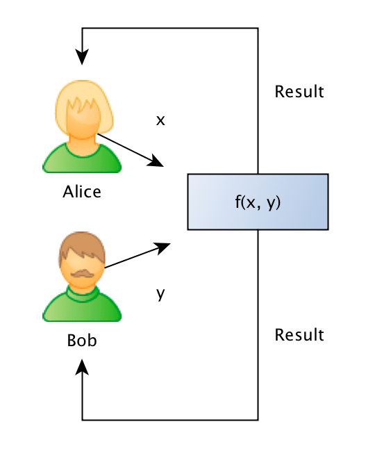
Formally what we want is to jointly evaluate the following function:
")
Such as the private values A and B are held private to the sole owner of it and where the result r will be known to just one or both of the parties.
It seems very counterintuitive that a problem like that could ever be solved, but for the surprise of many people, it is possible to solve it on some security requirements. Thanks to the recent developments in techniques such as FHE (Fully Homomorphic Encryption), Oblivious Transfer, Garbled Circuits, problems like that started to get practical for real-life usage and they are being nowadays being used by many companies in applications such as information exchange, secure location, advertisement, satellite orbit collision avoidance, etc.
I’m not going to enter into details of these techniques, but if you’re interested in the intuition behind the OT (Oblivious Transfer), you should definitely read the amazing explanation done by Craig Gidney here. There are also, of course, many different protocols for doing 2PC or MPC, where each one of them assumes some security requirements (semi-honest, malicious, etc), I’m not going to enter into the details to keep the post focused on the goal, but you should be aware of that.
The problem: sentence similarity
What we want to achieve is to use privacy-preserving computation to calculate the similarity between sentences without disclosing the content of the sentences. Just to give a concrete example: Bob owns a company and has the description of many different projects in sentences such as: “This project is about building a deep learning sentiment analysis framework that will be used for tweets“, and Alice who owns another competitor company, has also different projects described in similar sentences.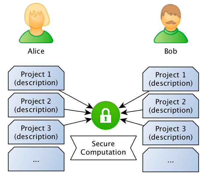 What they want to do is to jointly compute the similarity between projects in order to find if they should be doing partnership on a project or not, however, and this is the important point: Bob doesn’t want Alice to know the project descriptions and neither Alice wants Bob to be aware of their projects, they want to know the closest match between the different projects they run, but without disclosing the project ideas (project descriptions).
Sentence Similarity Comparison
Now, how can we exchange information about the Bob and Alice’s project sentences without disclosing information about the project descriptions ?
One naive way to do that would be to just compute the hashes of the sentences and then compare only the hashes to check if they match. However, this would assume that the descriptions are exactly the same, and besides that, if the entropy of the sentences is small (like small sentences), someone with reasonable computation power can try to recover the sentence.
Another approach for this problem (this is the approach that we’ll be using), is to compare the sentences in the sentence embeddings space. We just need to create sentence embeddings using a Machine Learning model (we’ll use InferSent later) and then compare the embeddings of the sentences. However, this approach also raises another concern: what if Bob or Alice trains a Seq2Seq model that would go from the embeddings of the other party back to an approximate description of the project ?
It isn’t unreasonable to think that one can recover an approximate description of the sentence given their embeddings. That’s why we’ll use the two-party secure computation for computing the embeddings similarity, in a way that Bob and Alice will compute the similarity of the embeddings without revealing their embeddings, keeping their project ideas safe.
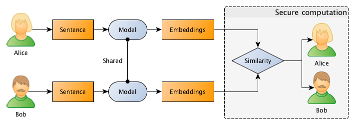
The entire flow is described in the image below, where Bob and Alice shares the same Machine Learning model, after that they use this model to go from sentences to embeddings, followed by a secure computation of the similarity in the embedding space.
Generating sentence embeddings with InferSent
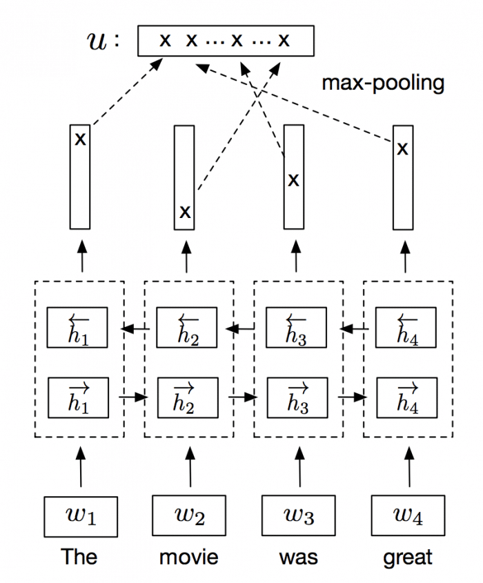
InferSent is an NLP technique for universal sentence representation developed by Facebook that uses supervised training to produce high transferable representations.
They used a Bi-directional LSTM with attention that consistently surpassed many unsupervised training methods such as the SkipThought vectors. They also provide a Pytorch implementation that we’ll use to generate sentence embeddings.
Note: even if you don’t have GPU, you can have reasonable performance doing embeddings for a few sentences.
The first step to generate the sentence embeddings is to download and load a pre-trained InferSent model:
import numpy as np
import torch

# Trained model from: https://github.com/facebookresearch/InferSent
GLOVE_EMBS = '../dataset/GloVe/glove.840B.300d.txt'
INFERSENT_MODEL = 'infersent.allnli.pickle'

# Load trained InferSent model
model = torch.load(INFERSENT_MODEL,
                   map_location=lambda storage, loc: storage)

model.set_glove_path(GLOVE_EMBS)
model.build_vocab_k_words(K=100000)
Now we need to define a similarity measure to compare two vectors, and for that goal, I’ll the cosine similarity (I wrote a tutorial about this similarity measure here) since it’s pretty straightforward:
 = \frac {\pmb x \cdot \pmb y}{||\pmb x|| \cdot ||\pmb y||}")
As you can see, if we have two unit vectors (vectors with norm 1), the two terms in the equation denominator will be 1 and we will be able to remove the entire denominator of the equation, leaving only:
 =\hat{x} \cdot\hat{y}")
So, if we normalize our vectors to have a unit norm (that’s why the vectors are wearing hats in the equation above), we can make the computation of the cosine similarity become just a simple dot product. That will help us a lot in computing the similarity distance later when we’ll use a framework to do the secure computation of this dot product.
So, the next step is to define a function that will take some sentence text and forward it to the model to generate the embeddings and then normalize them to unit vectors:
# This function will forward the text into the model and
# get the embeddings. After that, it will normalize it
# to a unit vector.

def encode(model, text):
    embedding = model.encode([text])[0]
    embedding /= np.linalg.norm(embedding)
    return embedding
As you can see, this function is pretty simple, it feeds the text into the model, and then it will divide the embedding vector by the embedding norm.
Now, for practical reasons, I’ll be using integer computation later for computing the similarity, however, the embeddings generated by InferSent are of course real values. For that reason, you’ll see in the code below that we create another function to scale the float values and remove the radix point and converting them to integers. There is also another important issue, the framework that we’ll be using later for secure computation doesn’t allow signed integers, so we also need to clip the embeddings values between 0.0 and 1.0. This will of course cause some approximation errors, however, we can still get very good approximations after clipping and scaling with limited precision (I’m using 14 bits for scaling to avoid overflow issues later during dot product computations):
# This function will scale the embedding in order to
# remove the radix point.

def scale(embedding):
    SCALE = 1 << 14
    scale_embedding = np.clip(embedding, 0.0, 1.0) * SCALE
    return scale_embedding.astype(np.int32)
You can use floating-point in your secure computations and there are a lot of frameworks that support them, however, it is more tricky to do that, and for that reason, I used integer arithmetic to simplify the tutorial. The function above is just a hack to make it simple. It’s easy to see that we can recover this embedding later without too much loss of precision.
Now we just need to create some sentence samples that we’ll be using:
# The list of Alice sentences
alice_sentences = [
    'my cat loves to walk over my keyboard',
    'I like to pet my cat',
]

# The list of Bob sentences
bob_sentences = [
    'the cat is always walking over my keyboard',
]
And convert them to embeddings:
# Alice sentences
alice_sentence1 = encode(model, alice_sentences[0])
alice_sentence2 = encode(model, alice_sentences[1])

# Bob sentences
bob_sentence1 = encode(model, bob_sentences[0])
Since we have now the sentences and every sentence is also normalized, we can compute cosine similarity just by doing a dot product between the vectors:
>>> np.dot(bob_sentence1, alice_sentence1)
0.8798542

>>> np.dot(bob_sentence1, alice_sentence2)
0.62976325
As we can see, the first sentence of Bob is most similar (~0.87) with Alice first sentence than to the Alice second sentence (~0.62).
Since we have now the embeddings, we just need to convert them to scaled integers:
# Scale the Alice sentence embeddings
alice_sentence1_scaled = scale(alice_sentence1)
alice_sentence2_scaled = scale(alice_sentence2)

# Scale the Bob sentence embeddings
bob_sentence1_scaled = scale(bob_sentence1)

# This is the unit vector embedding for the sentence
>>> alice_sentence1
array([ 0.01698913, -0.0014404 ,  0.0010993 , ...,  0.00252409,
        0.00828147,  0.00466533], dtype=float32)

# This is the scaled vector as integers
>>> alice_sentence1_scaled
array([278,   0,  18, ...,  41, 135,  76], dtype=int32)
Now with these embeddings as scaled integers, we can proceed to the second part, where we’ll be doing the secure computation between two parties.
Two-party secure computation
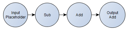
In order to perform secure computation between the two parties (Alice and Bob), we’ll use the ABY framework. ABY implements many difference secure computation schemes and allows you to describe your computation as a circuit like pictured in the image below, where the Yao’s Millionaire’s problem is described:
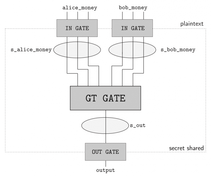
As you can see, we have two inputs entering in one GT GATE (greater than gate) and then a output. This circuit has a bit length of 3 for each input and will compute if the Alice input is greater than (GT GATE) the Bob input. The computing parties then secret share their private data and then can use arithmetic sharing, boolean sharing, or Yao sharing to securely evaluate these gates.
ABY is really easy to use because you can just describe your inputs, shares, gates and it will do the rest for you such as creating the socket communication channel, exchanging data when needed, etc. However, the implementation is entirely written in C++ and I’m not aware of any Python bindings for it (a great contribution opportunity).
Fortunately, there is an implemented example for ABY that can do dot product calculation for us, the example is here. I won’t replicate the example here, but the only part that we have to change is to read the embedding vectors that we created before instead of generating random vectors and increasing the bit length to 32-bits.
After that, we just need to execute the application on two different machines (or by emulating locally like below):
# This will execute the server part, the -r 0 specifies the role (server)
# and the -n 4096 defines the dimension of the vector (InferSent generates
# 4096-dimensional embeddings).
~# ./innerproduct -r 0 -n 4096

# And the same on another process (or another machine, however for another
# machine execution you'll have to obviously specify the IP).
~# ./innerproduct -r 1 -n 4096
And we get the following results:
Inner Product of alice_sentence1 and bob_sentence1  = 226691917
Inner Product of alice_sentence2 and bob_sentence1  = 171746521
Even in the integer representation, you can see that the inner product of the Alice’s first sentence and the Bob sentence is higher, meaning that the similarity is also higher. But let’s now convert this value back to float:
>>> SCALE = 1 << 14

# This is the dot product we should get
>>> np.dot(alice_sentence1, bob_sentence1)
0.8798542

# This is the inner product we got on secure computation
>>> 226691917 / SCALE**2.0
0.8444931

# This is the dot product we should get
>>> np.dot(alice_sentence2, bob_sentence1)
0.6297632

# This is the inner product we got on secure computation
>>> 171746521 / SCALE**2.0
0.6398056
As you can see, we got very good approximations, even in presence of low-precision math and unsigned integer requirements. Of course that in real-life you won’t have the two values and vectors, because they’re supposed to be hidden, but the changes to accommodate that are trivial, you just need to adjust ABY code to load only the vector of the party that it is executing it and using the correct IP addresses/port of the both parties.
I hope you liked it !
– Christian S. Perone


 the part 277,232,917 ends in 2 and when you subtract 1 you end up with 1 as the last digit, as you can confirm by looking at the
 that represents how much each pixel
  contributes to the output
  .
.


-5)+100)") , where I intentionally added redundant operations to see LLVM constant propagation later.
, where I intentionally added redundant operations to see LLVM constant propagation later.