I just tagged and released the v0.2 version of the Stallion. In the change log (Github project page), you can see that a lot of bugs were fixed and some new features were introduced in this release. I added compatibility with almost all Python 2.x versions, PyPy 1.7+ (and probably older versions too), I also fixed the compatibility with the Internet Explorer browser, now you should be able to use Stallion with Chrome, Firefox and IE.
The most important feature introduced is the global checking for updates (a lot of people requested it):
The new checking is under the menu “PyPI Repository”. Another new feature is the refactoring on the visual appearance of the package classifiers:
Some small visual enhancements were also introduced, like the little gray marker next to the selected package:
I hope you liked, I’m looking forward to implement more features as soon as possible, but a new version shouldn’t be released until next year.
Visit the project page at Github to get instructions on how to update or install Stallion.
I’m happy to announce the first release v.0.1 of the Stallion project. Stallion is a visual Python package manager compatible with Python 2.6 and 2.7 (I still haven’t tested it with Python 2.5).
The motivation behind Stallion is to provide an user friendly visualization with some management features (most of them are still under development) for Python packages installed on your local Python distribution. Stallion is intended to be used specially for Python newcomers.
The project is currently hosted at Github, so feel free to fork, contribute, make suggestion, report bugs, etc.
Installation
All you need to do to install Stallion is to use your favorite Python distribution system, examples:
user@machine:~/$ pip install stallion

or

user@machine:~/$ easy_install stallion
By doing this on your prompt (Windows/Linux), the pip/setuptools will download and install external dependencies (Flask, Jinja, docutils, etc.).
After installing Stallion, you need to start the local server by using:
user@machine:~/$ python -m stallion.main
And if it’s all ok, Stallion will start the server on localhost only at the port 5000, so all you need to do now is to browse into the URL http://localhost:5000
You can also download install packages from the PyPI repository.
You know, Python represents every object using the low-level C API PyObject (or PyVarObject for variable-size objects) structure, so, concretely, you can cast any Python object pointer to this type; this inheritance is built by hand, every new object must have a leading macro called PyObject_HEAD which defines the PyObject header for the object. The PyObject structure is declared in Include/object.h as:
… with two fields (forget the _PyObject_HEAD_EXTRA, it’s only used for a tracing debug feature) called ob_refcnt and ob_type, representing the reference counting for the object and the type of the object. I know you can use sys.getrefcount to get the reference counting of an object, but hacking the object memory using ctypes is by far more powerful, since you can get the contents of any field of the object (in cases where you don’t have a native API for that), I’ll show more examples later, but lets focus on the reference counting field of the object.
Getting the reference count (ob_refcnt)
So, in Python, we have the built-in function id(), this function returns the identity of the object, but, looking at its definition on CPython implementation, you’ll notice that id() returns the memory address of the object, see the source in Python/bltinmodule.c:
… the function PyLong_FromVoidPtr returns a Python long object from a void pointer. So, in CPython, this value is the address of the object in the memory as shown below:
[enlighter lang=”python”]
>>> value = 666
>>> hex(id(value))
‘0x8998e50’ # memory address of the ‘value’ object
[/enlighter]
Now that we have the memory address of the object, we can use the Python ctypes module to get the reference counting by accessing the attribute ob_refcnt, here is the code needed to do that:
What I’m doing here is getting the integer value from the ob_refcnt attribute of the PyObject in memory. Let’s add a new reference for the object ‘value’ we created, and then check the reference count again:
Note that the reference counting was increased by 1 due to the new reference variable called ‘value_ref’.
Interned strings state (ob_sstate)
Now, getting the reference count wasn’t even funny, we already had the sys.getrefcount API for that, but what about the interned state of the strings ? In order to avoid the creation of different allocations for the same string (and to speed comparisons), Python uses a dictionary that works like a “cache” for strings, this dictionary is defined in Objects/stringobject.c:
[enlighter lang=”c”]
/* This dictionary holds all interned strings. Note that references to
strings in this dictionary are *not* counted in the string’s ob_refcnt.
When the interned string reaches a refcnt of 0 the string deallocation
function will delete the reference from this dictionary.
Another way to look at this is that to say that the actual reference
count of a string is: s->ob_refcnt + (s->ob_sstate?2:0)
*/
static PyObject *interned;
[/enlighter]
I also copied here the comment about the dictionary, because is interesting to note that the strings in the dictionary aren’t counted in the string’s ob_refcnt.
So, the interned state of a string object is hold in the attribute ob_sstate of the string object, let’s see the definition of the Python string object:
[enlighter lang=”c”]
typedef struct {
PyObject_VAR_HEAD
long ob_shash;
int ob_sstate;
char ob_sval[1];
/* Invariants:
* ob_sval contains space for ‘ob_size+1’ elements.
* ob_sval[ob_size] == 0.
* ob_shash is the hash of the string or -1 if not computed yet.
* ob_sstate != 0 iff the string object is in stringobject.c’s
* ‘interned’ dictionary; in this case the two references
* from ‘interned’ to this object are *not counted* in ob_refcnt.
*/
} PyStringObject;
[/enlighter]
As you can note, strings objects inherit from the PyObject_VAR_HEAD macro, which defines another header attribute, let’s see the definition to get the complete idea of the structure:
[enlighter lang=”c”]
#define PyObject_VAR_HEAD \
PyObject_HEAD \
Py_ssize_t ob_size; /* Number of items in variable part */
[/enlighter]
The PyObject_VAR_HEAD macro adds another field called ob_size, which is the number of items on the variable part of the Python object (i.e. the number of items on a list object). So, before getting to the ob_sstate field, we need to shift our offset to skip the fields ob_refcnt (long), ob_type (void*) (from PyObject_HEAD), the field ob_size (long) (from PyObject_VAR_HEAD) and the field ob_shash(long) from the PyStringObject. Concretely, we need to skip this offset (3 fields with size long and one field with size void*) of bytes:
Now, let’s prepare two cases, one that we know that isn’t interned and another that is surely interned, then we’ll force the interned state of the other non-interned string to check the result of the ob_sstate attribute:
Note that the interned state for the object “a” is 1 and for the object “b” is 0. After forcing the interned state of the variable “b”, we can see that the field ob_sstate has changed to 1.
Changing internal states (evil mode)
Now, let’s suppose we want to change some internal state of a Python object through the interpreter. Let’s try to change the value of an int object. Int objects are defined in Include/intobject.h:
As you can see, the internal value of an int is stored in the field ob_ival, to change it, we just need to skip the ob_refcnt(long) and the ob_type (void*) from the PyObject_HEAD:
And that is it, we have changed the value of the int value directly in the memory.
I hope you liked it, you can play with lots of other Python objects like lists and dicts, note that this method is just intended to show how the Python objects are structured in the memory and how you can change them using the native API, but obviously, you’re not supposed to use this to change the value of ints lol.
Update 11/29/11: you’re not supposed to do such things on your production code or something like that, in this post I’m doing lazy assumptions about arch details like sizes of primitives, etc. Be warned.
This post is a continuation of the first part where we started to learn the theory and practice about text feature extraction and vector space model representation. I really recommend you to read the first part of the post series in order to follow this second post.
Since a lot of people liked the first part of this tutorial, this second part is a little longer than the first.
Introduction
In the first post, we learned how to use the term-frequency to represent textual information in the vector space. However, the main problem with the term-frequency approach is that it scales up frequent terms and scales down rare terms which are empirically more informative than the high frequency terms. The basic intuition is that a term that occurs frequently in many documents is not a good discriminator, and really makes sense (at least in many experimental tests); the important question here is: why would you, in a classification problem for instance, emphasize a term which is almost present in the entire corpus of your documents ?
The tf-idf weight comes to solve this problem. What tf-idf gives is how important is a word to a document in a collection, and that’s why tf-idf incorporates local and global parameters, because it takes in consideration not only the isolated term but also the term within the document collection. What tf-idf then does to solve that problem, is to scale down the frequent terms while scaling up the rare terms; a term that occurs 10 times more than another isn’t 10 times more important than it, that’s why tf-idf uses the logarithmic scale to do that.
But let’s go back to our definition of the which is actually the term count of the term in the document . The use of this simple term frequency could lead us to problems like keyword spamming, which is when we have a repeated term in a document with the purpose of improving its ranking on an IR (Information Retrieval) system or even create a bias towards long documents, making them look more important than they are just because of the high frequency of the term in the document.
To overcome this problem, the term frequency of a document on a vector space is usually also normalized. Let’s see how we normalize this vector.
Vector normalization
Suppose we are going to normalize the term-frequency vector that we have calculated in the first part of this tutorial. The document from the first part of this tutorial had this textual representation:
d4: We can see the shining sun, the bright sun.
And the vector space representation using the non-normalized term-frequency of that document was:
To normalize the vector, is the same as calculating the Unit Vector of the vector, and they are denoted using the “hat” notation: . The definition of the unit vector of a vector is:
Where the is the unit vector, or the normalized vector, the is the vector going to be normalized and the is the norm (magnitude, length) of the vector in the space (don’t worry, I’m going to explain it all).
The unit vector is actually nothing more than a normalized version of the vector, is a vector which the length is 1.
The normalization process (Source: http://processing.org/learning/pvector/)
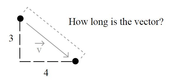
But the important question here is how the length of the vector is calculated and to understand this, you must understand the motivation of the spaces, also called Lebesgue spaces.
Lebesgue spaces
How long is this vector ? (Source: Source: http://processing.org/learning/pvector/)
Usually, the length of a vector is calculated using the Euclidean norm – a norm is a function that assigns a strictly positive length or size to all vectors in a vector space -, which is defined by:
(Source: http://processing.org/learning/pvector/)
But this isn’t the only way to define length, and that’s why you see (sometimes) a number together with the norm notation, like in . That’s because it could be generalized as:
and simplified as:
So when you read about a L2-norm, you’re reading about the Euclidean norm, a norm with , the most common norm used to measure the length of a vector, typically called “magnitude”; actually, when you have an unqualified length measure (without the number), you have the L2-norm (Euclidean norm).
When you read about a L1-norm, you’re reading about the norm with , defined as:
Which is nothing more than a simple sum of the components of the vector, also known as Taxicab distance, also called Manhattan distance.
Taxicab geometry versus Euclidean distance: In taxicab geometry all three pictured lines have the same length (12) for the same route. In Euclidean geometry, the green line has length , and is the unique shortest path.
Source: Wikipedia :: Taxicab Geometry
Note that you can also use any norm to normalize the vector, but we’re going to use the most common norm, the L2-Norm, which is also the default in the 0.9 release of the scikits.learn. You can also find papers comparing the performance of the two approaches among other methods to normalize the document vector, actually you can use any other method, but you have to be concise, once you’ve used a norm, you have to use it for the whole process directly involving the norm (a unit vector that used a L1-norm isn’t going to have the length 1 if you’re going to take its L2-norm later).
Back to vector normalization
Now that you know what the vector normalization process is, we can try a concrete example, the process of using the L2-norm (we’ll use the right terms now) to normalize our vector in order to get its unit vector . To do that, we’ll simple plug it into the definition of the unit vector to evaluate it:
And that is it ! Our normalized vector has now a L2-norm .
Note that here we have normalized our term frequency document vector, but later we’re going to do that after the calculation of the tf-idf.
The term frequency – inverse document frequency (tf-idf) weight
Now you have understood how the vector normalization works in theory and practice, let’s continue our tutorial. Suppose you have the following documents in your collection (taken from the first part of tutorial):
Train Document Set:

d1: The sky is blue.
d2: The sun is bright.

Test Document Set:

d3: The sun in the sky is bright.
d4: We can see the shining sun, the bright sun.
Your document space can be defined then as where is the number of documents in your corpus, and in our case as and . The cardinality of our document space is defined by and , since we have only 2 two documents for training and testing, but they obviously don’t need to have the same cardinality.
Let’s see now, how idf (inverse document frequency) is then defined:
where is the number of documents where the term appears, when the term-frequency function satisfies , we’re only adding 1 into the formula to avoid zero-division.
The formula for the tf-idf is then:
and this formula has an important consequence: a high weight of the tf-idf calculation is reached when you have a high term frequency (tf) in the given document (local parameter) and a low document frequency of the term in the whole collection (global parameter).
Now let’s calculate the idf for each feature present in the feature matrix with the term frequency we have calculated in the first tutorial:
Since we have 4 features, we have to calculate , , , :
These idf weights can be represented by a vector as:
Now that we have our matrix with the term frequency () and the vector representing the idf for each feature of our matrix (), we can calculate our tf-idf weights. What we have to do is a simple multiplication of each column of the matrix with the respective vector dimension. To do that, we can create a square diagonal matrix called with both the vertical and horizontal dimensions equal to the vector dimension:
and then multiply it to the term frequency matrix, so the final result can be defined then as:
Please note that the matrix multiplication isn’t commutative, the result of will be different than the result of the , and this is why the is on the right side of the multiplication, to accomplish the desired effect of multiplying each idf value to its corresponding feature:
Let’s see now a concrete example of this multiplication:
And finally, we can apply our L2 normalization process to the matrix. Please note that this normalization is “row-wise” because we’re going to handle each row of the matrix as a separated vector to be normalized, and not the matrix as a whole:
And that is our pretty normalized tf-idf weight of our testing document set, which is actually a collection of unit vectors. If you take the L2-norm of each row of the matrix, you’ll see that they all have a L2-norm of 1.
Now the section you were waiting for ! In this section I’ll use Python to show each step of the tf-idf calculation using the Scikit.learn feature extraction module.
The first step is to create our training and testing document set and computing the term frequency matrix:
from sklearn.feature_extraction.text import CountVectorizer

train_set = ("The sky is blue.", "The sun is bright.")
test_set = ("The sun in the sky is bright.",
"We can see the shining sun, the bright sun.")

count_vectorizer = CountVectorizer()
count_vectorizer.fit_transform(train_set)
print "Vocabulary:", count_vectorizer.vocabulary

# Vocabulary: {'blue': 0, 'sun': 1, 'bright': 2, 'sky': 3}

freq_term_matrix = count_vectorizer.transform(test_set)
print freq_term_matrix.todense()

#[[0 1 1 1]
#[0 2 1 0]]
Now that we have the frequency term matrix (called freq_term_matrix), we can instantiate the TfidfTransformer, which is going to be responsible to calculate the tf-idf weights for our term frequency matrix:
Note that I’ve specified the norm as L2, this is optional (actually the default is L2-norm), but I’ve added the parameter to make it explicit to you that it it’s going to use the L2-norm. Also note that you can see the calculated idf weight by accessing the internal attribute called idf_. Now that fit() method has calculated the idf for the matrix, let’s transform the freq_term_matrix to the tf-idf weight matrix:
And that is it, the tf_idf_matrix is actually our previous matrix. You can accomplish the same effect by using the Vectorizer class of the Scikit.learn which is a vectorizer that automatically combines the CountVectorizer and the TfidfTransformer to you. See this example to know how to use it for the text classification process.
I really hope you liked the post, I tried to make it simple as possible even for people without the required mathematical background of linear algebra, etc. In the next Machine Learning post I’m expecting to show how you can use the tf-idf to calculate the cosine similarity.
If you liked it, feel free to comment and make suggestions, corrections, etc.
What I’ve built to consider these questions is an interactive robotic painting machine that uses artificial intelligence to paint its own body of work and to make its own decisions. While doing so, it listens to its environment and considers what it hears as input into the painting process. In the absence of someone or something else making sound in its presence, the machine, like many artists, listens to itself. But when it does hear others, it changes what it does just as we subtly (or not so subtly) are influenced by what others tell us.
The aim of this post is to show to the reader how to plot the recent Japan earthquake data from the USGS using the pyearthquake module. If you want to know more information about the pyearthquakemodule, take a look in this post where I previously used it. pyearthquake is a pure-python module which exposes an API to retrieve data from the USGS site as well from the MODIS Rapid Response System (recently, they created a separate project to handle Japan daily images).
Installing pyearthquake
The first thing we need to do is to install the Python pyearthquake module, you can do it using easy_install from setuptools:
easy_install pyearthquake
The easy_install should automatically handle the required modules, but if you face problems (specially in Ubuntu with basemap, here is the version requirements: matplotlib >= 0.99.0, numpy >= 1.3.0, PIL >= 1.1.6 and basemap >= 0.99.4.
In that context, we have 1179 incidents with magnitude 1+ from the past 7 days.
Lets filter now only events with magnitude 6+, which represents the recent significant earthquakes:
>>> mag6_list = [event for event in catalog if float(event["Magnitude"]) >= 6.0]
>>> len(mag6_list)
30
We have now 30 events with magnitude 6+ from the past 7 days, let’s print it:
>>> for row in mag6_list:
...    print row["Eqid"], row["Magnitude"], row["Depth"],
...          row["Datetime"], row["Depth"], row["Region"]
...
c0001z5z 6.3 8.70 Friday, March 11, 2011 20:11:22 UTC 8.70 near the east coast of Honshu, Japan
c0001z4n 6.6 10.00 Friday, March 11, 2011 19:46:49 UTC 10.00 near the west coast of Honshu, Japan
c0001z2t 6.1 24.80 Friday, March 11, 2011 19:02:58 UTC 24.80 near the east coast of Honshu, Japan
c0001z2a 6.2 10.00 Friday, March 11, 2011 18:59:15 UTC 10.00 near the west coast of Honshu, Japan
c0001yib 6.2 18.90 Friday, March 11, 2011 15:13:14 UTC 18.90 near the east coast of Honshu, Japan
c0001y4u 6.5 11.60 Friday, March 11, 2011 11:36:39 UTC 11.60 near the east coast of Honshu, Japan
(...)
As you can see, almost all last events are earthquakes from the Japan coast. Here, you can extract any individual event and retrieve USGS products like ShakeMaps, etc (see more information in this post on how to fetch and show those USGS products).
Plotting events into the map
Now we will plot those events into the map (pyearthquake uses the matplotlib toolkit called basemap to plot events into the map):
>>> usgs.plot_events(catalog)
The “catalog” variable is the same we retrieved before using the USGS M1+PAST_7DAY catalog.
Here is what what this statement will show:
Now we can zoom into Japan using the button , and this is the result:
The colored dots are the events from the retrieved catalog, the more strong the color the more strong was the earthquake; see the dark red color near the cost, that event was the unfortunate and catastrophic 8.9 magnitude earthquake which devastated Japan yesterday.
Retrieving near real-time MODIS Rapid Response images
MODIS has processed image subsets of Aqua and Terra satellites. One of these subsets is called “japan” and it has the entire country coverage. Let’s retrieve this MODIS subset and then plot our events in this same map:
What pyearthquake is going to do here is to download (this may take some time) the entire subset for the resolution of 250m (the best available), parse the subset metadata, align image into the map between the lat/lng bounds and then plot the events over this satellite image, so we’ll have the last high resolution satellite images from the Japan together with the earthquake events plot, and here is the result:
If you are going to PyCon US 2011, I would like to invite you to the talk “Genetic Programming in Python“, the talk will be given by Eric Floehr on March 12th 1:20 p.m. – 2:05 p.m.
Here is the abstract:
Did you know you can create and evolve programs that find solutions to problems? This talk walks through how to use Genetic Algorithms and Genetic Programming as tools to discover solutions to hard problems, when to use GA/GP, setting up the GA/GP environment, and interpreting the results. Using pyevolve, we’ll walk through a real-world implementation creating a GP that predicts the weather.
(…)
Genetic Algorithms (GA) and Genetic Programming (GP) are methods used to search for and optimize solutions in large solution spaces. GA/GP use concepts borrowed from natural evolution, such as mutation, cross-over, selection, population, and fitness to generate solutions to problems. If done well, these solutions will become better as the GA/GP runs.
GA/GP has been used in problem domains as diverse as scheduling, database index optimization, circuit board layout, mirror and lens design, game strategies, and robotic walking and swimming. They can also be a lot of fun, and have been used to evolve aesthetically pleasing artwork, melodies, and approximating pictures or paintings using polygons.
GA/GP is fun to play with because often-times an unexpected solution will be created that will give new insight or knowledge. It might also present a novel solution to a problem, one that a human may never generate. Solutions may also be inscrutable, and determining why a solution works is interesting in itself.
This website uses cookies to improve your experience. We'll assume you're ok with this, but you can opt-out if you wish. Cookie settingsACCEPT
Privacy & Cookies Policy
Privacy Overview
This website uses cookies to improve your experience while you navigate through the website. Out of these cookies, the cookies that are categorized as necessary are stored on your browser as they are essential for the working of basic functionalities of the website. We also use third-party cookies that help us analyze and understand how you use this website. These cookies will be stored in your browser only with your consent. You also have the option to opt-out of these cookies. But opting out of some of these cookies may have an effect on your browsing experience.
Necessary cookies are absolutely essential for the website to function properly. This category only includes cookies that ensures basic functionalities and security features of the website. These cookies do not store any personal information.
Any cookies that may not be particularly necessary for the website to function and is used specifically to collect user personal data via analytics, ads, other embedded contents are termed as non-necessary cookies. It is mandatory to procure user consent prior to running these cookies on your website.


") which is actually the term count of the term
which is actually the term count of the term  in the document
  . The use of this simple term frequency could lead us to problems like keyword spamming, which is when we have a repeated term in a document with the purpose of improving its ranking on an IR (Information Retrieval) system or even create a bias towards long documents, making them look more important than they are just because of the high frequency of the term in the document.
 that we have calculated in the first part of this tutorial. The document
  from the first part of this tutorial had this textual representation:
")
 . The definition of the unit vector
  is:
is:
 is the norm (magnitude, length) of the vector
  space (don’t worry, I’m going to explain it all).
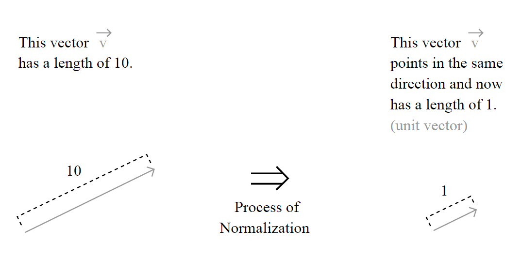
") is calculated using the
is calculated using the 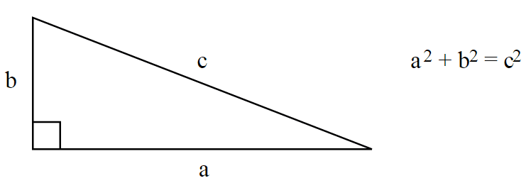

 together with the norm notation, like in
  . That’s because it could be generalized as:
^\frac{1}{p}")
^\frac{1}{p}")
 , the most common norm used to measure the length of a vector, typically called “magnitude”; actually, when you have an unqualified length measure (without the
  , defined as:
")

 , and is the unique shortest path.
 . To do that, we’ll simple plug it into the definition of the unit vector to evaluate it:
}{\sqrt{0^2 + 2^2 + 1^2 + 0^2}} \\ \\ \hat{v_{d_4}} = \frac{(0,2,1,0)}{\sqrt{5}} \\ \\ \small \hat{v_{d_4}} = (0.0, 0.89442719, 0.4472136, 0.0)")
 .
. where
where  is the number of documents in your corpus, and in our case as
  and
and  . The cardinality of our document space is defined by
  and
and  , since we have only 2 two documents for training and testing, but they obviously don’t need to have the same cardinality.
 = \log{\frac{\left|D\right|}{1+\left|\{d : t \in d\}\right|}}")
 is the number of documents where the term
  \neq 0") , we’re only adding 1 into the formula to avoid zero-division.
, we’re only adding 1 into the formula to avoid zero-division. = \mathrm{tf}(t, d) \times \mathrm{idf}(t)")

") ,
, ") ,
, ") ,
, ") :
: = \log{\frac{\left|D\right|}{1+\left|\{d : t_1 \in d\}\right|}} = \log{\frac{2}{1}} = 0.69314718")
 = \log{\frac{\left|D\right|}{1+\left|\{d : t_2 \in d\}\right|}} = \log{\frac{2}{3}} = -0.40546511")
 = \log{\frac{\left|D\right|}{1+\left|\{d : t_3 \in d\}\right|}} = \log{\frac{2}{3}} = -0.40546511")
 = \log{\frac{\left|D\right|}{1+\left|\{d : t_4 \in d\}\right|}} = \log{\frac{2}{2}} = 0.0")
")
 ) and the vector representing the idf for each feature of our matrix (
 ), we can calculate our tf-idf weights. What we have to do is a simple multiplication of each column of the matrix
  with both the vertical and horizontal dimensions equal to the vector

 will be different than the result of the
  , and this is why the
  & \mathrm{tf}(t_2, d_1) & \mathrm{tf}(t_3, d_1) & \mathrm{tf}(t_4, d_1)\\ \mathrm{tf}(t_1, d_2) & \mathrm{tf}(t_2, d_2) & \mathrm{tf}(t_3, d_2) & \mathrm{tf}(t_4, d_2) \end{bmatrix} \times \begin{bmatrix} \mathrm{idf}(t_1) & 0 & 0 & 0\\ 0 & \mathrm{idf}(t_2) & 0 & 0\\ 0 & 0 & \mathrm{idf}(t_3) & 0\\ 0 & 0 & 0 & \mathrm{idf}(t_4) \end{bmatrix} \\ = \begin{bmatrix} \mathrm{tf}(t_1, d_1) \times \mathrm{idf}(t_1) & \mathrm{tf}(t_2, d_1) \times \mathrm{idf}(t_2) & \mathrm{tf}(t_3, d_1) \times \mathrm{idf}(t_3) & \mathrm{tf}(t_4, d_1) \times \mathrm{idf}(t_4)\\ \mathrm{tf}(t_1, d_2) \times \mathrm{idf}(t_1) & \mathrm{tf}(t_2, d_2) \times \mathrm{idf}(t_2) & \mathrm{tf}(t_3, d_2) \times \mathrm{idf}(t_3) & \mathrm{tf}(t_4, d_2) \times \mathrm{idf}(t_4) \end{bmatrix}")

 matrix. Please note that this normalization is “row-wise” because we’re going to handle each row of the matrix as a separated vector to be normalized, and not the matrix as a whole:


