Update 17/01: reddit discussion thread.
Update 19/01: hacker news thread.
The codex
 The Voynich Manuscript is a hand-written codex written in an unknown system and carbon-dated to the early 15th century (1404–1438). Although the manuscript has been studied by some famous cryptographers of the World War I and II, nobody has deciphered it yet. The manuscript is known to be written in two different languages (Language A and Language B) and it is also known to be written by a group of people. The manuscript itself is always subject of a lot of different hypothesis, including the one that I like the most which is the “culture extinction” hypothesis, supported in 2014 by Stephen Bax. This hypothesis states that the codex isn’t ciphered, it states that the codex was just written in an unknown language that disappeared due to a culture extinction. In 2014, Stephen Bax proposed a provisional, partial decoding of the manuscript, the video of his presentation is very interesting and I really recommend you to watch if you like this codex. There is also a transcription of the manuscript done thanks to the hard-work of many folks working on it since many moons ago.
Word vectors
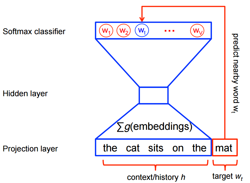
My idea when I heard about the work of Stephen Bax was to try to capture the patterns of the text using word2vec. Word embeddings are created by using a shallow neural network architecture. It is a unsupervised technique that uses supervided learning tasks to learn the linguistic context of the words. Here is a visualization of this architecture from the TensorFlow site:
These word vectors, after trained, carry with them a lot of semantic meaning. For instance:
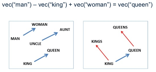
We can see that those vectors can be used in vector operations to extract information about the regularities of the captured linguistic semantics. These vectors also approximates same-meaning words together, allowing similarity queries like in the example below:
>>> model.most_similar("man")
[(u'woman', 0.6056041121482849), (u'guy', 0.4935004413127899), (u'boy', 0.48933547735214233), (u'men', 0.4632953703403473), (u'person', 0.45742249488830566), (u'lady', 0.4487500488758087), (u'himself', 0.4288588762283325), (u'girl', 0.4166809320449829), (u'his', 0.3853422999382019), (u'he', 0.38293731212615967)]

>>> model.most_similar("queen")
[(u'princess', 0.519856333732605), (u'latifah', 0.47644317150115967), (u'prince', 0.45914226770401), (u'king', 0.4466976821422577), (u'elizabeth', 0.4134873151779175), (u'antoinette', 0.41033703088760376), (u'marie', 0.4061327874660492), (u'stepmother', 0.4040161967277527), (u'belle', 0.38827288150787354), (u'lovely', 0.38668593764305115)]
Word vectors can also be used (surprise) for translation, and this is the feature of the word vectors that I think that its most important when used to understand text where we know some of the words translations. I pretend to try to use the words found by Stephen Bax in the future to check if it is possible to capture some transformation that could lead to find similar structures with other languages. A nice visualization of this feature is the one below from the paper “Exploiting Similarities among Languages for Machine Translation“:
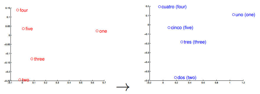
This visualization was made using gradient descent to optimize a linear transformation between the source and destination language word vectors. As you can see, the structure in Spanish is really close to the structure in English.
EVA Transcription
To train this model, I had to parse and extract the transcription from the EVA (European Voynich Alphabet) to be able to feed the Voynich sentences into the word2vec model. This EVA transcription has the following format:
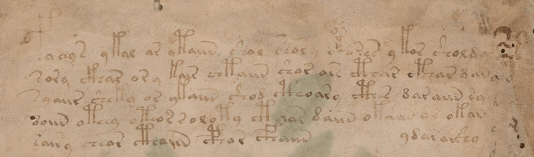
<f1r.P1.1;H>       fachys.ykal.ar.ataiin.shol.shory.cth!res.y.kor.sholdy!-
<f1r.P1.1;C>       fachys.ykal.ar.ataiin.shol.shory.cthorys.y.kor.sholdy!-
<f1r.P1.1;F>       fya!ys.ykal.ar.ytaiin.shol.shory.*k*!res.y!kor.sholdy!-
<f1r.P1.1;N>       fachys.ykal.ar.ataiin.shol.shory.cth!res.y,kor.sholdy!-
<f1r.P1.1;U>       fya!ys.ykal.ar.ytaiin.shol.shory.***!r*s.y.kor.sholdo*-
#
<f1r.P1.2;H>       sory.ckhar.o!r.y.kair.chtaiin.shar.are.cthar.cthar.dan!-
<f1r.P1.2;C>       sory.ckhar.o.r.y.kain.shtaiin.shar.ar*.cthar.cthar.dan!-
<f1r.P1.2;F>       sory.ckhar.o!r!y.kair.chtaiin.shor.ar!.cthar.cthar.dana-
<f1r.P1.2;N>       sory.ckhar.o!r,y.kair.chtaiin.shar.are.cthar.cthar,dan!-
<f1r.P1.2;U>       sory.ckhar.o!r!y.kair.chtaiin.shor.ary.cthar.cthar.dan*-
The first data between “<” and “>” has information about the folio (page), line and author of the transcription. The transcription block above is the transcription for the first two lines of the first folio of the manuscript below:
As you can see, the EVA contains some code characters, like for instance “!”, “*” and they all have some meaning, like to inform that the author doing that translation is not sure about the character in that position, etc. EVA also contains transcription from different authors for the same line of the folio.
To convert this transcription to sentences I used only lines where the authors were sure about the entire line and I used the first line where the line satisfied this condition. I also did some cleaning on the transcription to remove the drawings names from the text, like: “text.text.text-{plant}text” -> “text text texttext”.
After this conversion from the EVA transcript to sentences compatible with the word2vec model, I trained the model to provide 100-dimensional word vectors for the words of the manuscript.
Vector space visualizations using t-SNE
After training word vectors, I created a visualization of the 100-dimensional vectors into a 2D embedding space using t-SNE algorithm:
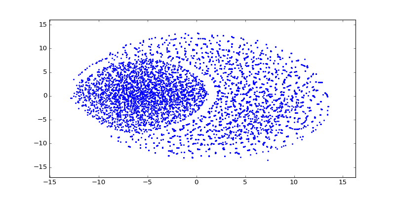
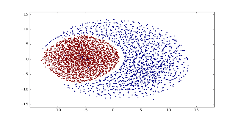
As you can see there are a lot of small clusters and there visually two big clusters, probably accounting for the two different languages used in the Codex (I still need to confirm this regarding the two languages aspect). After clustering it with DBSCAN (using the original word vectors, not the t-SNE transformed vectors), we can clearly see the two major clusters:
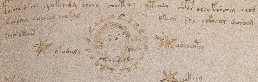
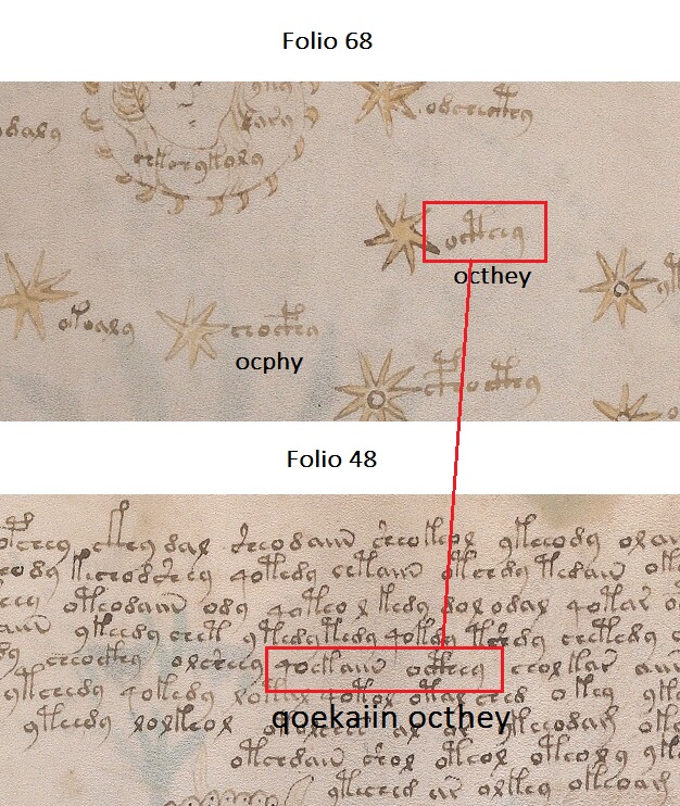
Now comes the really interesting and useful part of the word vectors, if use a star name from the folio below (it’s pretty obvious why it is know that this is probably a star name):
>>> w2v_model.most_similar("octhey")

[('qoekaiin', 0.6402825713157654),
 ('otcheody', 0.6389687061309814),
 ('ytchos', 0.566596269607544),
 ('ocphy', 0.5415685176849365),
 ('dolchedy', 0.5343093872070312),
 ('aiicthy', 0.5323750376701355),
 ('odchecthy', 0.5235849022865295),
 ('okeeos', 0.5187858939170837),
 ('cphocthy', 0.5159749388694763),
 ('oteor', 0.5050544738769531)]
I get really interesting similar words, like for instance the ocphy and other close star names:
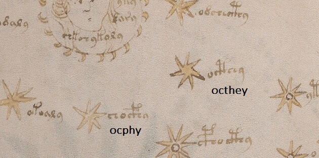
It also returns the word “qoekaiin” from the folio 48, that precedes the same star name:
As you can see, word vectors are really useful to find some linguistic structures, we can also create another plot, showing how close are the star names in the 2D embedding space visualization created using t-SNE:
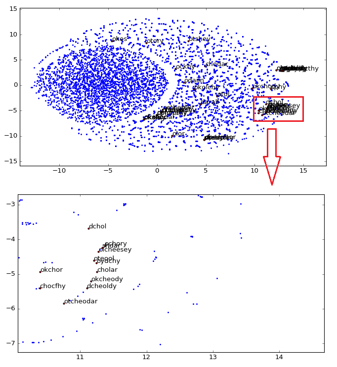
As you can see, we zoomed the major cluster of stars and we can see that they are really all grouped together in the vector space. These representations can be used for instance to infer plat names from the herbal section, etc.
My idea was to show how useful word vectors are to analyze unknown codex texts, I hope you liked and I hope that this could be somehow useful for other people how are also interested in this amazing manuscript.
– Christian S. Perone

") and
and ") , where
, where  and
and  are the components of the vector (features of the document, or TF-IDF values for each word of the document in our example) and the
  is the dimension of the vectors:
 \\ \vec{b} = (4, 0) \\ \vec{a} \cdot \vec{b} = 0*4 + 3*0 = 0")


 ? This term is the projection of the vector
  into the vector
  as shown on the image below:

 :
:


 ) and move the
  to the right hand of the equation:
 is the same as the inverse of the cosine (
 ).
).") which is actually the term count of the term
which is actually the term count of the term  in the document
  . The use of this simple term frequency could lead us to problems like keyword spamming, which is when we have a repeated term in a document with the purpose of improving its ranking on an IR (Information Retrieval) system or even create a bias towards long documents, making them look more important than they are just because of the high frequency of the term in the document.
 that we have calculated in the first part of this tutorial. The document
  from the first part of this tutorial had this textual representation:
")
 . The definition of the unit vector
  is:
is:
 is the norm (magnitude, length) of the vector
  space (don’t worry, I’m going to explain it all).
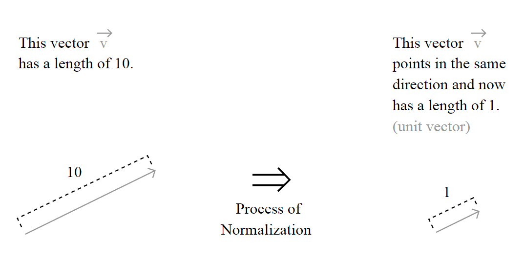
") is calculated using the
is calculated using the 

 together with the norm notation, like in
  . That’s because it could be generalized as:
^\frac{1}{p}")
^\frac{1}{p}")
 , the most common norm used to measure the length of a vector, typically called “magnitude”; actually, when you have an unqualified length measure (without the
  , defined as:
")

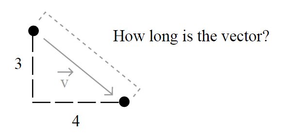
 , and is the unique shortest path.
 . To do that, we’ll simple plug it into the definition of the unit vector to evaluate it:
}{\sqrt{0^2 + 2^2 + 1^2 + 0^2}} \\ \\ \hat{v_{d_4}} = \frac{(0,2,1,0)}{\sqrt{5}} \\ \\ \small \hat{v_{d_4}} = (0.0, 0.89442719, 0.4472136, 0.0)")
 .
. where
where  is the number of documents in your corpus, and in our case as
  and
and  . The cardinality of our document space is defined by
  and
and  , since we have only 2 two documents for training and testing, but they obviously don’t need to have the same cardinality.
 = \log{\frac{\left|D\right|}{1+\left|\{d : t \in d\}\right|}}")
 is the number of documents where the term
  \neq 0") , we’re only adding 1 into the formula to avoid zero-division.
, we’re only adding 1 into the formula to avoid zero-division. = \mathrm{tf}(t, d) \times \mathrm{idf}(t)")

") ,
, ") ,
, ") ,
, ") :
: = \log{\frac{\left|D\right|}{1+\left|\{d : t_1 \in d\}\right|}} = \log{\frac{2}{1}} = 0.69314718")
 = \log{\frac{\left|D\right|}{1+\left|\{d : t_2 \in d\}\right|}} = \log{\frac{2}{3}} = -0.40546511")
 = \log{\frac{\left|D\right|}{1+\left|\{d : t_3 \in d\}\right|}} = \log{\frac{2}{3}} = -0.40546511")
 = \log{\frac{\left|D\right|}{1+\left|\{d : t_4 \in d\}\right|}} = \log{\frac{2}{2}} = 0.0")
")
 ) and the vector representing the idf for each feature of our matrix (
 ), we can calculate our tf-idf weights. What we have to do is a simple multiplication of each column of the matrix
  with both the vertical and horizontal dimensions equal to the vector

 will be different than the result of the
  , and this is why the
  & \mathrm{tf}(t_2, d_1) & \mathrm{tf}(t_3, d_1) & \mathrm{tf}(t_4, d_1)\\ \mathrm{tf}(t_1, d_2) & \mathrm{tf}(t_2, d_2) & \mathrm{tf}(t_3, d_2) & \mathrm{tf}(t_4, d_2) \end{bmatrix} \times \begin{bmatrix} \mathrm{idf}(t_1) & 0 & 0 & 0\\ 0 & \mathrm{idf}(t_2) & 0 & 0\\ 0 & 0 & \mathrm{idf}(t_3) & 0\\ 0 & 0 & 0 & \mathrm{idf}(t_4) \end{bmatrix} \\ = \begin{bmatrix} \mathrm{tf}(t_1, d_1) \times \mathrm{idf}(t_1) & \mathrm{tf}(t_2, d_1) \times \mathrm{idf}(t_2) & \mathrm{tf}(t_3, d_1) \times \mathrm{idf}(t_3) & \mathrm{tf}(t_4, d_1) \times \mathrm{idf}(t_4)\\ \mathrm{tf}(t_1, d_2) \times \mathrm{idf}(t_1) & \mathrm{tf}(t_2, d_2) \times \mathrm{idf}(t_2) & \mathrm{tf}(t_3, d_2) \times \mathrm{idf}(t_3) & \mathrm{tf}(t_4, d_2) \times \mathrm{idf}(t_4) \end{bmatrix}")

 matrix. Please note that this normalization is “row-wise” because we’re going to handle each row of the matrix as a separated vector to be normalized, and not the matrix as a whole:

 and
and  from the document set, we’ll have the following index vocabulary denoted as
 ") where the
where the  = \begin{cases} 1, & \mbox{if } t\mbox{ is \"blue\"} \\ 2, & \mbox{if } t\mbox{ is \"sun\"} \\ 3, & \mbox{if } t\mbox{ is \"bright\"} \\ 4, & \mbox{if } t\mbox{ is \"sky\"} \\ \end{cases}")
 or
or  = \sum\limits_{x\in d} \mathrm{fr}(x, t)")
") is a simple function defined as:
is a simple function defined as: = \begin{cases} 1, & \mbox{if } x = t \\ 0, & \mbox{otherwise} \\ \end{cases}")
") returns is how many times is the term
returns is how many times is the term  = 2") since we have only two occurrences of the term “sun” in the document
since we have only two occurrences of the term “sun” in the document , \mathrm{tf}(t_2,d_n), \mathrm{tf}(t_3,d_n), \ldots, \mathrm{tf}(t_n,d_n))")
") represents the frequency-term of the term 1 or
represents the frequency-term of the term 1 or  (which is our “blue” term of the vocabulary) in the document
  .
. and
and  are represented as vectors:
, \mathrm{tf}(t_2,d_3), \mathrm{tf}(t_3,d_3), \ldots, \mathrm{tf}(t_n,d_3)) \\ \vec{v_{d_4}} = (\mathrm{tf}(t_1,d_4), \mathrm{tf}(t_2,d_4), \mathrm{tf}(t_3,d_4), \ldots, \mathrm{tf}(t_n,d_4))")
 \\ \vec{v_{d_4}} = (0, 2, 1, 0)")
 shows that we have, in order, 0 occurrences of the term “blue”, 1 occurrence of the term “sun”, and so on. In the
  shape, where
  is the cardinality of the document space, or how many documents we have and the
  is the number of features, in our case represented by the vocabulary size. An example of the matrix representation of the vectors described above is:
") (except because it is zero-indexed).
(except because it is zero-indexed). we cited earlier in this post, which represents the two document vectors