I just published the slides of the talk below presented at the Machine Learning Porto Alegre meetup in Brazil:
by Christian S. Perone
I just published the slides of the talk below presented at the Machine Learning Porto Alegre meetup in Brazil:
Training neural networks is often done by measuring many different metrics such as accuracy, loss, gradients, etc. This is most of the time done aggregating these metrics and plotting visualizations on TensorBoard.
 There are, however, other senses that we can use to monitor the training of neural networks, such as sound. Sound is one of the perspectives that is currently very poorly explored in the training of neural networks. Human hearing can be very good a distinguishing very small perturbations in characteristics such as rhythm and pitch, even when these perturbations are very short in time or subtle.
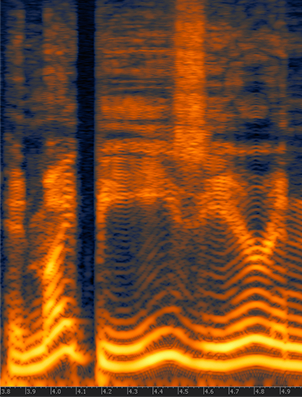
For this experiment, I made a very simple example showing a synthesized sound that was made using the gradient norm of each layer and for step of the training for a convolutional neural network training on MNIST using different settings such as different learning rates, optimizers, momentum, etc.
You’ll need to install PyAudio and PyTorch to run the code (in the end of this post).
This segment represents a training session with gradients from 4 layers during the first 200 steps of the first epoch and using a batch size of 10. The higher the pitch, the higher the norm for a layer, there is a short silence to indicate different batches. Note the gradient increasing during time.
Same as above, but with higher learning rate.
Same as above, but with high learning rate that makes the network to diverge, pay attention to the high pitch when the norms explode and then divergence.
Same setting but with a high learning rate of 1.0 and a batch size of 256. Note how the gradients explode and then there are NaNs causing the final sound.
This is using Adam in the same setting as the SGD.
For those who are interested, here is the entire source code I used to make the sound clips:
import pyaudio
import numpy as np
import wave

import torch
import torch.nn as nn
import torch.nn.functional as F
import torch.optim as optim
from torchvision import datasets, transforms


class Net(nn.Module):
    def __init__(self):
        super(Net, self).__init__()
        self.conv1 = nn.Conv2d(1, 20, 5, 1)
        self.conv2 = nn.Conv2d(20, 50, 5, 1)
        self.fc1 = nn.Linear(4*4*50, 500)
        self.fc2 = nn.Linear(500, 10)

        self.ordered_layers = [self.conv1,
                               self.conv2,
                               self.fc1,
                               self.fc2]

    def forward(self, x):
        x = F.relu(self.conv1(x))
        x = F.max_pool2d(x, 2, 2)
        x = F.relu(self.conv2(x))
        x = F.max_pool2d(x, 2, 2)
        x = x.view(-1, 4*4*50)
        x = F.relu(self.fc1(x))
        x = self.fc2(x)
        return F.log_softmax(x, dim=1)


def open_stream(fs):
    p = pyaudio.PyAudio()
    stream = p.open(format=pyaudio.paFloat32,
                    channels=1,
                    rate=fs,
                    output=True)
    return p, stream


def generate_tone(fs, freq, duration):
    npsin = np.sin(2 * np.pi * np.arange(fs*duration) * freq / fs)
    samples = npsin.astype(np.float32)
    return 0.1 * samples


def train(model, device, train_loader, optimizer, epoch):
    model.train()

    fs = 44100
    duration = 0.01
    f = 200.0
    p, stream = open_stream(fs)

    frames = []

    for batch_idx, (data, target) in enumerate(train_loader):
        data, target = data.to(device), target.to(device)
        optimizer.zero_grad()
        output = model(data)
        loss = F.nll_loss(output, target)
        loss.backward()

        norms = []
        for layer in model.ordered_layers:
            norm_grad = layer.weight.grad.norm()
            norms.append(norm_grad)

            tone = f + ((norm_grad.numpy()) * 100.0)
            tone = tone.astype(np.float32)
            samples = generate_tone(fs, tone, duration)

            frames.append(samples)

        silence = np.zeros(samples.shape[0] * 2,
                           dtype=np.float32)
        frames.append(silence)

        optimizer.step()

        # Just 200 steps per epoach
        if batch_idx == 200:
            break

    wf = wave.open("sgd_lr_1_0_bs256.wav", 'wb')
    wf.setnchannels(1)
    wf.setsampwidth(p.get_sample_size(pyaudio.paFloat32))
    wf.setframerate(fs)
    wf.writeframes(b''.join(frames))
    wf.close()

    stream.stop_stream()
    stream.close()
    p.terminate()


def run_main():
    device = torch.device("cpu")

    train_loader = torch.utils.data.DataLoader(
        datasets.MNIST('../data', train=True, download=True,
                       transform=transforms.Compose([
                           transforms.ToTensor(),
                           transforms.Normalize((0.1307,), (0.3081,))
                       ])),
        batch_size=256, shuffle=True)

    model = Net().to(device)
    optimizer = optim.SGD(model.parameters(), lr=0.01, momentum=0.5)

    for epoch in range(1, 2):
        train(model, device, train_loader, optimizer, epoch)


if __name__ == "__main__":
    run_main()
Just sharing some slides I presented at the PyData Lisbon on July 2019 about the talk “Uncertainty Estimation in Deep Learning“:
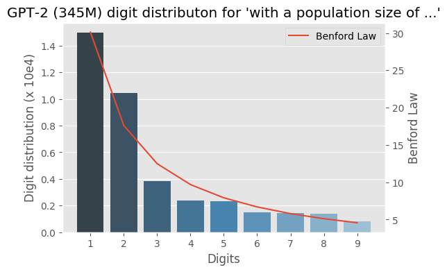
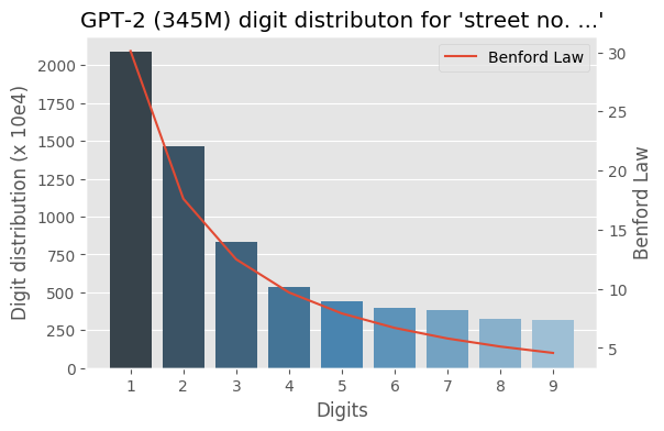
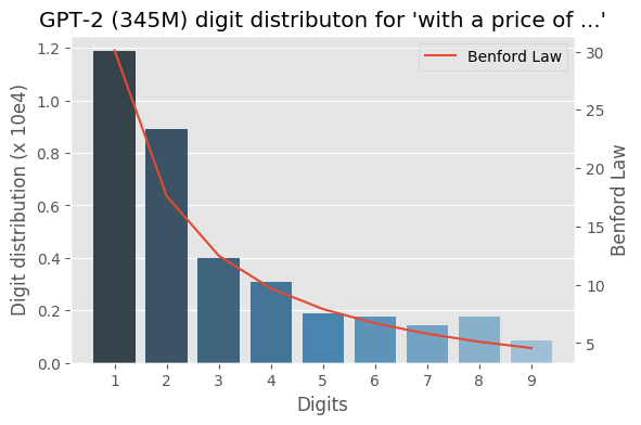
I wrote some months ago about how the Benford law emerges from language models, today I decided to evaluate the same method to check how the GPT-2 would behave with some sentences and it turns out that it seems that it is also capturing these power laws. You can find some plots with the examples below, the plots are showing the probability of the digit given a particular sentence such as “with a population size of”, showing the distribution of: $$P(\{1,2, \ldots, 9\} \vert \text{“with a population size of”})$$ for the GPT-2 medium model (345M):
I was experimenting with the approach described in “Randomized Prior Functions for Deep Reinforcement Learning” by Ian Osband et al. at NPS 2018, where they devised a very simple and practical method for uncertainty using bootstrap and randomized priors and decided to share the PyTorch code.
I really like bootstrap approaches, and in my opinion, they are usually the easiest methods to implement and provide very good posterior approximation with deep connections to Bayesian approaches, without having to deal with variational inference. They actually show in the paper that in the linear case, the method provides a Bayes posterior.
The main idea of the method is to have bootstrap to provide a non-parametric data perturbation together with randomized priors, which are nothing more than just random initialized networks.
$$Q_{\theta_k}(x) = f_{\theta_k}(x) + p_k(x)$$
The final model \(Q_{\theta_k}(x)\) will be the k model of the ensemble that will fit the function \(f_{\theta_k}(x)\) with an untrained prior \(p_k(x)\).
Let’s go to the code. The first class is a simple MLP with 2 hidden layers and Glorot initialization :
class MLP(nn.Module):
    def __init__(self):
        super().__init__()
        self.l1 = nn.Linear(1, 20)
        self.l2 = nn.Linear(20, 20)
        self.l3 = nn.Linear(20, 1)

        nn.init.xavier_uniform_(self.l1.weight)
        nn.init.xavier_uniform_(self.l2.weight)
        nn.init.xavier_uniform_(self.l3.weight)

    def forward(self, inputs):
        x = self.l1(inputs)
        x = nn.functional.selu(x)
        x = self.l2(x)
        x = nn.functional.selu(x)
        x = self.l3(x)
        return x
Then later we define a class that will take the model and the prior to produce the final model result:
class ModelWithPrior(nn.Module):
    def __init__(self,
                 base_model : nn.Module,
                 prior_model : nn.Module,
                 prior_scale : float = 1.0):
        super().__init__()
        self.base_model = base_model
        self.prior_model = prior_model
        self.prior_scale = prior_scale

    def forward(self, inputs):
        with torch.no_grad():
            prior_out = self.prior_model(inputs)
            prior_out = prior_out.detach()
        model_out = self.base_model(inputs)
        return model_out + (self.prior_scale * prior_out)
And it’s basically that ! As you can see, it’s a very simple method, in the second part we just created a custom forward() to avoid computing/accumulating gradients for the prior network and them summing (after scaling) it with the model prediction.
To train it, you just have to use different bootstraps for each ensemble model, like in the code below:
def train_model(x_train, y_train, base_model, prior_model):
    model = ModelWithPrior(base_model, prior_model, 1.0)
    loss_fn = nn.MSELoss()
    optimizer = torch.optim.Adam(model.parameters(), lr=0.05)

    for epoch in range(100):
        model.train()
        preds = model(x_train)
        loss = loss_fn(preds, y_train)

        optimizer.zero_grad()
        loss.backward()
        optimizer.step()

    return model
and using a sampler with replacement (bootstrap) as in:
dataset = TensorDataset(...)
bootstrap_sampler = RandomSampler(dataset, True, len(dataset))
train_dataloader = DataLoader(dataset,
                              batch_size=len(dataset),
                              sampler=bootstrap_sampler)
In this case, I used the same small dataset used in the original paper: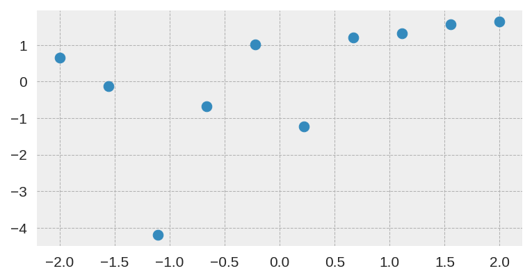
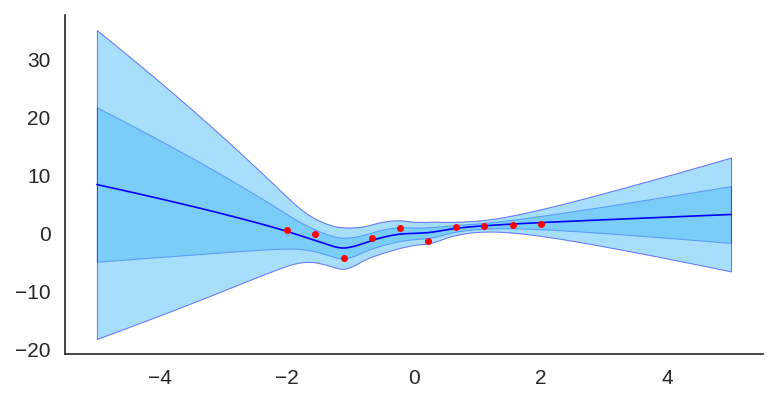
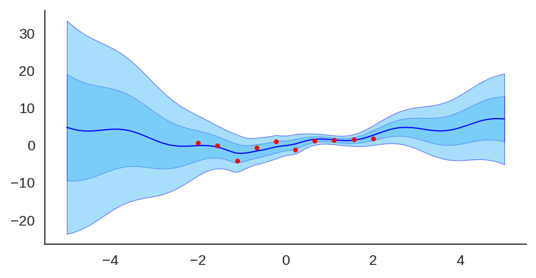
After training it with a simple MLP prior as well, the results for the uncertainty are shown below:
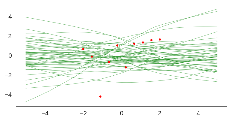
If we look at just the priors, we will see the variation of the untrained networks:
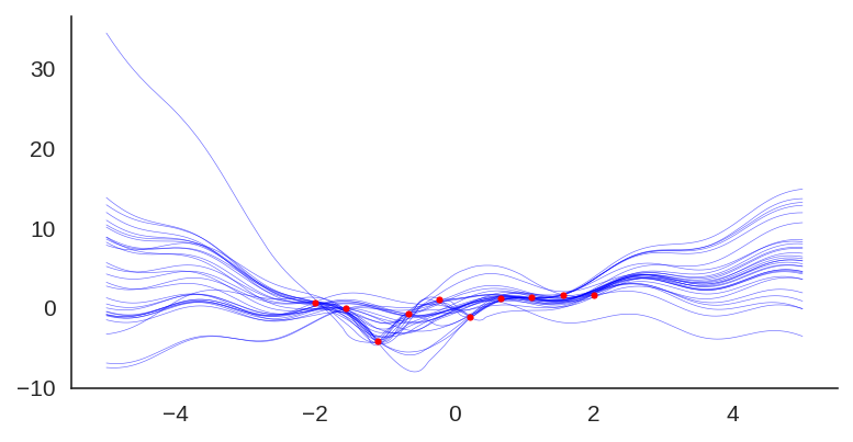
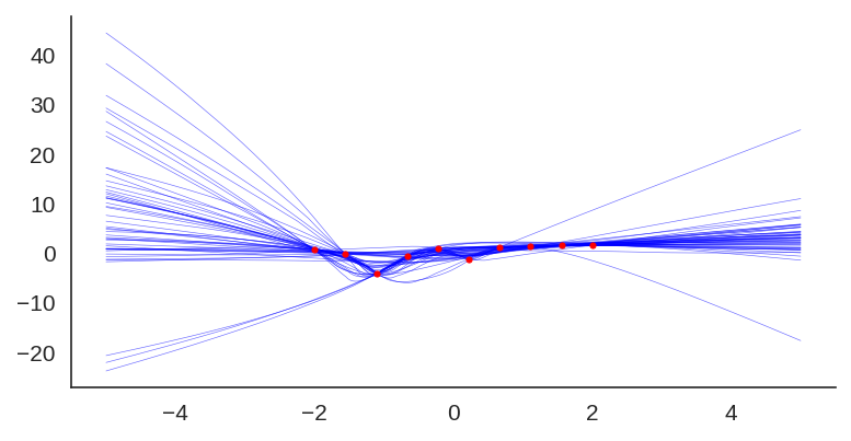
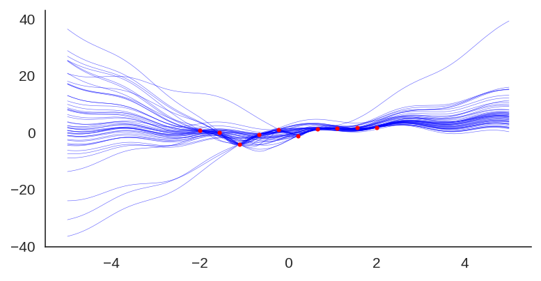
We can also visualize the individual model predictions showing their variability due to different initializations as well as the bootstrap noise:
Now, what is also quite interesting, is that we can change the prior to let’s say a fixed sine:
class SinPrior(nn.Module):
    def forward(self, input):
        return torch.sin(3 * input)
Then, when we train the same MLP model but this time using the sine prior, we can see how it affects the final prediction and uncertainty bounds:
If we show each individual model, we can see the effect of the prior contribution to each individual model:
I hope you liked, these are quite amazing results for a simple method that at least pass the linear “sanity check”. I’ll explore some pre-trained networks in place of the prior to see the different effects on predictions, it’s a very interesting way to add some simple priors.
These are the slides of the talk I presented on PyData Montreal on Feb 25th. It was a pleasure to meet you all ! Thanks a lot to Maria and Alexander for the invitation !
It is frustrating to learn about principles such as maximum likelihood estimation (MLE), maximum a posteriori (MAP) and Bayesian inference in general. The main reason behind this difficulty, in my opinion, is that many tutorials assume previous knowledge, use implicit or inconsistent notation, or are even addressing a completely different concept, thus overloading these principles.
Those aforementioned issues make it very confusing for newcomers to understand these concepts, and I’m often confronted by people who were unfortunately misled by many tutorials. For that reason, I decided to write a sane introduction to these concepts and elaborate more on their relationships and hidden interactions while trying to explain every step of formulations. I hope to bring something new to help people understand these principles.
The maximum likelihood estimation is a method or principle used to estimate the parameter or parameters of a model given observation or observations. Maximum likelihood estimation is also abbreviated as MLE, and it is also known as the method of maximum likelihood. From this name, you probably already understood that this principle works by maximizing the likelihood, therefore, the key to understand the maximum likelihood estimation is to first understand what is a likelihood and why someone would want to maximize it in order to estimate model parameters.
Let’s start with the definition of the likelihood function for continuous case:
$$\mathcal{L}(\theta | x) = p_{\theta}(x)$$
The left term means “the likelihood of the parameters \(\theta\), given data \(x\)”. Now, what does that mean ? It means that in the continuous case, the likelihood of the model \(p_{\theta}(x)\) with the parametrization \(\theta\) and data \(x\) is the probability density function (pdf) of the model with that particular parametrization.
Although this is the most used likelihood representation, you should pay attention that the notation \(\mathcal{L}(\cdot | \cdot)\) in this case doesn’t mean the same as the conditional notation, so be careful with this overload, because it is always implicitly stated and it is also often a source of confusion. Another representation of the likelihood that is often used is \(\mathcal{L}(x; \theta)\), which is better in the sense that it makes it clear that it’s not a conditional, however, it makes it look like the likelihood is a function of the data and not of the parameters.
The model \(p_{\theta}(x)\) can be any distribution, and to make things concrete, let’s say that we are assuming that the data generating distribution is an univariate Gaussian distribution, which we define below:
$$
\begin{align}
p(x) & \sim \mathcal{N}(\mu, \sigma^2) \\
p(x; \mu, \sigma^2) & \sim \frac{1}{\sqrt{2\pi\sigma^2}} \exp{ \bigg[-\frac{1}{2}\bigg( \frac{x-\mu}{\sigma}\bigg)^2 \bigg] }
\end{align}
$$
If you plot this probability density function with different parametrizations, you’ll get something like the plots below, where the red distribution is the standard Gaussian \(p(x) \sim \mathcal{N}(0, 1.0)\):
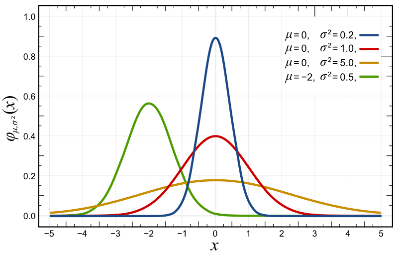
As you can see in the probability density function (pdf) plot above, the likelihood of \(x\) at variously given realizations are showed in the y-axis. Another source of confusion here is that usually, people take this as a probability, because they usually see these plots of normals and the likelihood is always below 1, however, the probability density function doesn’t give you probabilities but densities. The constraint on the pdf is that it must integrate to one:
$$\int_{-\infty}^{+\infty} f(x)dx = 1$$
So, it is completely normal to have densities larger than 1 in many points for many different distributions. Take for example the pdf for the Beta distribution below:
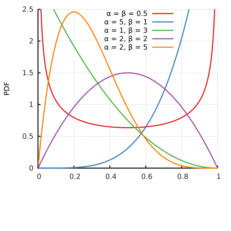
As you can see, the pdf shows densities above one in many parametrizations of the distribution, while still integrating into 1 and following the second axiom of probability: the unit measure.
So, returning to our original principle of maximum likelihood estimation, what we want is to maximize the likelihood \(\mathcal{L}(\theta | x)\) for our observed data. What this means in practical terms is that we want to find the parameters \(\theta\) of our model where the likelihood that this model generated our data is maximized, we want to find which parameters of this model are most plausible to have generated this observed data, or what are the parameters that make this sample most probable ?
For the case of our univariate Gaussian model, what we want is to find the parameters \(\mu\) and \(\sigma^2\), which for convenient notation we collapse into a single parameter vector:
$$\theta = \begin{bmatrix}\mu \\ \sigma^2\end{bmatrix}$$
Because these are the statistics that completely define our univariate Gaussian model. So let’s formulate the problem of the maximum likelihood estimation:
$$
\begin{align}
\hat{\theta} &= \mathrm{arg}\max_\theta \mathcal{L}(\theta | x) \\
&= \mathrm{arg}\max_\theta p_{\theta}(x)
\end{align}
$$
This says that we want to obtain the maximum likelihood estimate \(\hat{\theta}\) that approximates \(p_{\theta}(x)\) to a underlying “true” distribution \(p_{\theta^*}(x)\) by maximizing the likelihood of the parameters \(\theta\) given data \(x\). You shouldn’t confuse a maximum likelihood estimate \(\hat{\theta}(x)\) which is a realization of the maximum likelihood estimator for the data \(x\), with the maximum likelihood estimator \(\hat{\theta}\), so pay attention to disambiguate it in your head.
However, we need to incorporate multiple observations in this formulation, and by adding multiple observations we end up with a complex joint distribution:
$$\hat{\theta} = \mathrm{arg}\max_\theta p_{\theta}(x_1, x_2, \ldots, x_n)$$
That needs to take into account the interactions between all observations. And here is where we make a strong assumption: we state that the observations are independent. Independent random variables mean that the following holds:
$$p_{\theta}(x_1, x_2, \ldots, x_n) = \prod_{i=1}^{n} p_{\theta}(x_i)$$
Which means that since \(x_1, x_2, \ldots, x_n\) don’t contain information about each other, we can write the joint probability as a product of their marginals.
Another assumption that is made, is that these random variables are identically distributed, which means that they came from the same generating distribution, which allows us to model it with the same distribution parametrization.
Given these two assumptions, which are also known as IID (independently and identically distributed), we can formulate our maximum likelihood estimation problem as:
$$\hat{\theta} = \mathrm{arg}\max_\theta \prod_{i=1}^{n} p_{\theta}(x_i)$$
Note that MLE doesn’t require you to make these assumptions, however, many problems will appear if you don’t to it, such as different distributions for each sample or having to deal with joint probabilities.
Given that in many cases these densities that we multiply can be very small, multiplying one by the other in the product that we have above we can end up with very small values. Here is where the logarithm function makes its way to the likelihood. The log function is a strictly monotonically increasing function, that preserves the location of the extrema and has a very nice property:
$$\log ab = \log a + \log b $$
Where the logarithm of a product is the sum of the logarithms, which is very convenient for us, so we’ll apply the logarithm to the likelihood to maximize what is called the log-likelihood:
$$
\begin{align}
\hat{\theta} &= \mathrm{arg}\max_\theta \prod_{i=1}^{n} p_{\theta}(x_i) \\
&= \mathrm{arg}\max_\theta \sum_{i=1}^{n} \log p_{\theta}(x_i) \\
\end{align}
$$
As you can see, we went from a product to a summation, which is much more convenient. Another reason for the application of the logarithm is that we often take the derivative and solve it for the parameters, therefore is much easier to work with a summation than a multiplication.
We can also conveniently average the log-likelihood (given that we’re just including a multiplication by a constant):
$$
\begin{align}
\hat{\theta} &= \mathrm{arg}\max_\theta \sum_{i=1}^{n} \log p_{\theta}(x_i) \\
&= \mathrm{arg}\max_\theta \frac{1}{n} \sum_{i=1}^{n} \log p_{\theta}(x_i) \\
\end{align}
$$
This is also convenient because it will take out the dependency on the number of observations. We also know, that through the law of large numbers, the following holds as \(n\to\infty\):
$$
\frac{1}{n} \sum_{i=1}^{n} \log \, p_{\theta}(x_i) \approx \mathbb{E}_{x \sim p_{\theta^*}(x)}\left[\log \, p_{\theta}(x) \right]
$$
As you can see, we’re approximating the expectation with the empirical expectation defined by our dataset \(\{x_i\}_{i=1}^{n}\). This is an important point and it is usually implictly assumed.
The weak law of large numbers can be bounded using a Chebyshev bound, and if you are interested in concentration inequalities, I’ve made an article about them here where I discuss the Chebyshev bound.
To finish our formulation, given that we usually minimize objectives, we can formulate the same maximum likelihood estimation as the minimization of the negative of the log-likelihood:
$$
\hat{\theta} = \mathrm{arg}\min_\theta -\mathbb{E}_{x \sim p_{\theta^*}(x)}\left[\log \, p_{\theta}(x) \right]
$$
Which is exactly the same thing with just the negation turn the maximization problem into a minimization problem.
It is well-known that maximizing the likelihood is the same as minimizing the Kullback-Leibler divergence, also known as the KL divergence. Which is very interesting because it links a measure from information theory with the maximum likelihood principle.
The KL divergence is defined as:
$$
\begin{equation}
D_{KL}( p || q)=\int p(x)\log\frac{p(x)}{q(x)} \ dx
\end{equation}
$$
There are many intuitions to understand the KL divergence, I personally like the perspective on the likelihood ratios, however, there are plenty of materials about it that you can easily find and it’s out of the scope of this introduction.
The KL divergence is basically the expectation of the log-likelihood ratio under the \(p(x)\) distribution. What we’re doing below is just rephrasing it by using some identities and properties of the expectation:
$$
\begin{align}
D_{KL}[p_{\theta^*}(x) \, \Vert \, p_\theta(x)] &= \mathbb{E}_{x \sim p_{\theta^*}(x)}\left[\log \frac{p_{\theta^*}(x)}{p_\theta(x)} \right] \\
\label{eq:logquotient}
&= \mathbb{E}_{x \sim p_{\theta^*}(x)}\left[\log \,p_{\theta^*}(x) – \log \, p_\theta(x) \right] \\
\label{eq:linearization}
&= \mathbb{E}_{x \sim p_{\theta^*}(x)} \underbrace{\left[\log \, p_{\theta^*}(x) \right]}_{\text{Entropy of } p_{\theta^*}(x)} – \underbrace{\mathbb{E}_{x \sim p_{\theta^*}(x)}\left[\log \, p_{\theta}(x) \right]}_{\text{Negative of log-likelihood}}
\end{align}
$$
In the formulation above, we’re first using the fact that the logarithm of a quotient is equal to the difference of the logs of the numerator and denominator (equation \(\ref{eq:logquotient}\)). After that we use the linearization of the expectation(equation \(\ref{eq:linearization}\)), which tells us that \(\mathbb{E}\left[X + Y\right] = \mathbb{E}\left[X\right]+\mathbb{E}\left[Y\right]\). In the end, we are left with two terms, the first one in the left is the entropy and the one in the right you can recognize as the negative of the log-likelihood that we saw earlier.
If we want to minimize the KL divergence for the \(\theta\), we can ignore the first term, since it doesn’t depend of \(\theta\) in any way, and in the end we have exactly the same maximum likelihood formulation that we saw before:
$$
\begin{eqnarray}
\require{cancel}
\theta^* &=& \mathrm{arg}\min_\theta \cancel{\mathbb{E}_{x \sim p_{\theta^*}(x)} \left[\log \, p_{\theta^*}(x) \right]} – \mathbb{E}_{x \sim p_{\theta^*}(x)}\left[\log \, p_{\theta}(x) \right]\\
&=& \mathrm{arg}\min_\theta -\mathbb{E}_{x \sim p_{\theta^*}(x)}\left[\log \, p_{\theta}(x) \right]
\end{eqnarray}
$$
A very common scenario in Machine Learning is supervised learning, where we have data points \(x_n\) and their labels \(y_n\) building up our dataset \( D = \{ (x_1, y_1), (x_2, y_2), \ldots, (x_n, y_n) \} \), where we’re interested in estimating the conditional probability of \(\textbf{y}\) given \(\textbf{x}\), or more precisely \( P_{\theta}(Y | X) \).
To extend the maximum likelihood principle to the conditional case, we just have to write it as:
$$
\hat{\theta} = \mathrm{arg}\min_\theta -\mathbb{E}_{x \sim p_{\theta^*}(y | x)}\left[\log \, p_{\theta}(y | x) \right]
$$
And then it can be easily generalized to formulate the linear regression:
$$
p_{\theta}(y | x) \sim \mathcal{N}(x^T \theta, \sigma^2) \\
\log p_{\theta}(y | x) = -n \log \sigma – \frac{n}{2} \log{2\pi} – \sum_{i=1}^{n}{\frac{\| x_i^T \theta – y_i \|}{2\sigma^2}}
$$
In that case, you can see that we end up with a sum of squared errors that will have the same location of the optimum of the mean squared error (MSE). So you can see that minimizing the MSE is equivalent of maximizing the likelihood for a Gaussian model.
The maximum likelihood estimation has very interesting properties but it gives us only point estimates, and this means that we cannot reason on the distribution of these estimates. In contrast, Bayesian inference can give us a full distribution over parameters, and therefore will allow us to reason about the posterior distribution.
I’ll write more about Bayesian inference and sampling methods such as the ones from the Markov Chain Monte Carlo (MCMC) family, but I’ll leave this for another article, right now I’ll continue showing the relationship of the maximum likelihood estimator with the maximum a posteriori (MAP) estimator.
Although the maximum a posteriori, also known as MAP, also provides us with a point estimate, it is a Bayesian concept that incorporates a prior over the parameters. We’ll also see that the MAP has a strong connection with the regularized MLE estimation.
We know from the Bayes rule that we can get the posterior from the product of the likelihood and the prior, normalized by the evidence:
$$
\begin{align}
p(\theta \vert x) &= \frac{p_{\theta}(x) p(\theta)}{p(x)} \\
\label{eq:proport}
&\propto p_{\theta}(x) p(\theta)
\end{align}
$$
In the equation \(\ref{eq:proport}\), since we’re worried about optimization, we cancel the normalizing evidence \(p(x)\) and stay with a proportional posterior, which is very convenient because the marginalization of \(p(x)\) involves integration and is intractable for many cases.
$$
\begin{align}
\theta_{MAP} &= \mathop{\rm arg\,max}\limits_{\theta} p_{\theta}(x) p(\theta) \\
&= \mathop{\rm arg\,max}\limits_{\theta} \prod_{i=1}^{n} p_{\theta}(x_i) p(\theta) \\
&= \mathop{\rm arg\,max}\limits_{\theta} \sum_{i=1}^{n} \underbrace{\log p_{\theta}(x_i)}_{\text{Log likelihood}} \underbrace{p(\theta)}_{\text{Prior}}
\end{align}
$$
In this formulation above, we just followed the same steps as described earlier for the maximum likelihood estimator, we assume independence and an identical distributional setting, followed later by the logarithm application to switch from a product to a summation. As you can see in the final formulation, this is equivalent as the maximum likelihood estimation multiplied by the prior term.
We can also easily recover the exact maximum likelihood estimator by using a uniform prior \(p(\theta) \sim \textbf{U}(\cdot, \cdot)\). This means that every possible value of \(\theta\) will be equally weighted, meaning that it’s just a constant multiplication:
$$
\begin{align}
\theta_{MAP} &= \mathop{\rm arg\,max}\limits_{\theta} \sum_i \log p_{\theta}(x_i) p(\theta) \\
&= \mathop{\rm arg\,max}\limits_{\theta} \sum_i \log p_{\theta}(x_i) \, \text{constant} \\
&= \underbrace{\mathop{\rm arg\,max}\limits_{\theta} \sum_i \log p_{\theta}(x_i)}_{\text{Equivalent to maximum likelihood estimation (MLE)}} \\
\end{align}
$$
And there you are, the MAP with a uniform prior is equivalent to MLE. It is also easy to show that a Gaussian prior can recover the L2 regularized MLE. Which is quite interesting, given that it can provide insights and a new perspective on the regularization terms that we usually use.
I hope you liked this article ! The next one will be about Bayesian inference with posterior sampling, where we’ll show how we can reason about the posterior distribution and not only on point estimates as seen in MAP and MLE.
– Christian S. Perone
![]()
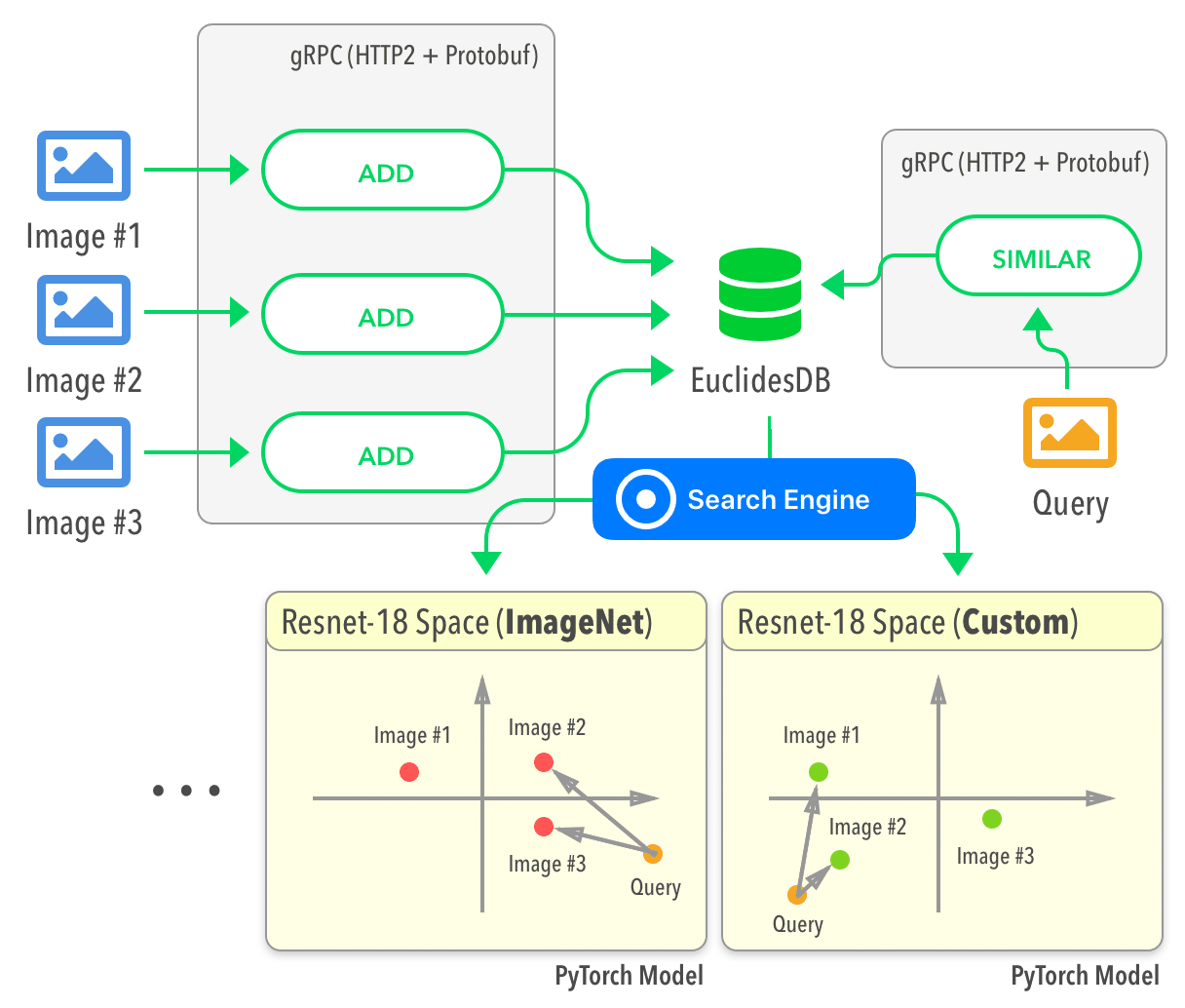
Past week I released the first public version of EuclidesDB. EuclidesDB is a multi-model machine learning feature database that is tightly coupled with PyTorch and provides a backend for including and querying data on the model feature space.
For more information, see the GitHub repository or the documentation.
Some features of EuclidesDB are listed below:
And here is a diagram of the overall architecture: