Randomized prior functions in PyTorch
I was experimenting with the approach described in “Randomized Prior Functions for Deep Reinforcement Learning” by Ian Osband et al. at NPS 2018, where they devised a very simple and practical method for uncertainty using bootstrap and randomized priors and decided to share the PyTorch code.
I really like bootstrap approaches, and in my opinion, they are usually the easiest methods to implement and provide very good posterior approximation with deep connections to Bayesian approaches, without having to deal with variational inference. They actually show in the paper that in the linear case, the method provides a Bayes posterior.
The main idea of the method is to have bootstrap to provide a non-parametric data perturbation together with randomized priors, which are nothing more than just random initialized networks.
$$Q_{\theta_k}(x) = f_{\theta_k}(x) + p_k(x)$$
The final model \(Q_{\theta_k}(x)\) will be the k model of the ensemble that will fit the function \(f_{\theta_k}(x)\) with an untrained prior \(p_k(x)\).
Let’s go to the code. The first class is a simple MLP with 2 hidden layers and Glorot initialization :
class MLP(nn.Module):
    def __init__(self):
        super().__init__()
        self.l1 = nn.Linear(1, 20)
        self.l2 = nn.Linear(20, 20)
        self.l3 = nn.Linear(20, 1)

        nn.init.xavier_uniform_(self.l1.weight)
        nn.init.xavier_uniform_(self.l2.weight)
        nn.init.xavier_uniform_(self.l3.weight)

    def forward(self, inputs):
        x = self.l1(inputs)
        x = nn.functional.selu(x)
        x = self.l2(x)
        x = nn.functional.selu(x)
        x = self.l3(x)
        return x
Then later we define a class that will take the model and the prior to produce the final model result:
class ModelWithPrior(nn.Module):
    def __init__(self,
                 base_model : nn.Module,
                 prior_model : nn.Module,
                 prior_scale : float = 1.0):
        super().__init__()
        self.base_model = base_model
        self.prior_model = prior_model
        self.prior_scale = prior_scale

    def forward(self, inputs):
        with torch.no_grad():
            prior_out = self.prior_model(inputs)
            prior_out = prior_out.detach()
        model_out = self.base_model(inputs)
        return model_out + (self.prior_scale * prior_out)
And it’s basically that ! As you can see, it’s a very simple method, in the second part we just created a custom forward() to avoid computing/accumulating gradients for the prior network and them summing (after scaling) it with the model prediction.
To train it, you just have to use different bootstraps for each ensemble model, like in the code below:
def train_model(x_train, y_train, base_model, prior_model):
    model = ModelWithPrior(base_model, prior_model, 1.0)
    loss_fn = nn.MSELoss()
    optimizer = torch.optim.Adam(model.parameters(), lr=0.05)

    for epoch in range(100):
        model.train()
        preds = model(x_train)
        loss = loss_fn(preds, y_train)

        optimizer.zero_grad()
        loss.backward()
        optimizer.step()

    return model
and using a sampler with replacement (bootstrap) as in:
dataset = TensorDataset(...)
bootstrap_sampler = RandomSampler(dataset, True, len(dataset))
train_dataloader = DataLoader(dataset,
                              batch_size=len(dataset),
                              sampler=bootstrap_sampler)
In this case, I used the same small dataset used in the original paper: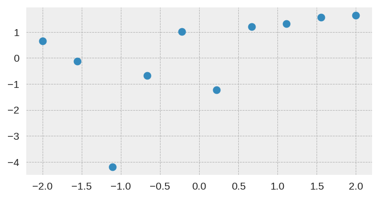
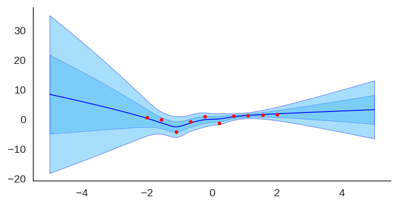
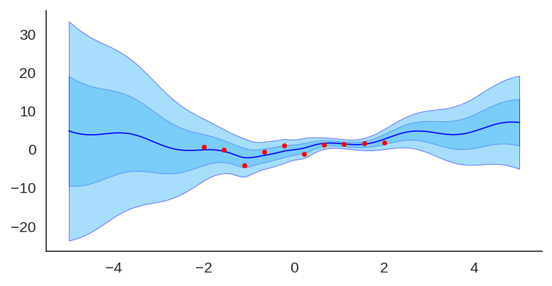
After training it with a simple MLP prior as well, the results for the uncertainty are shown below:
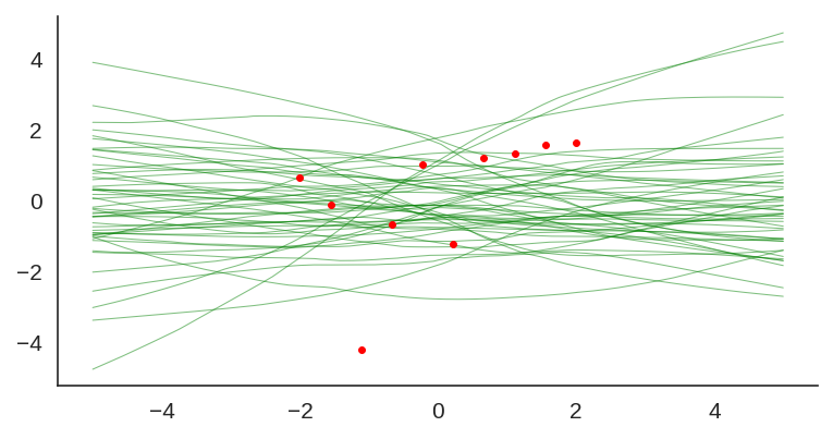
If we look at just the priors, we will see the variation of the untrained networks:
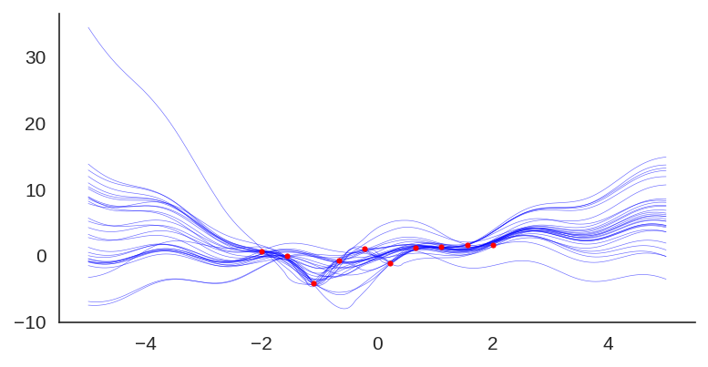
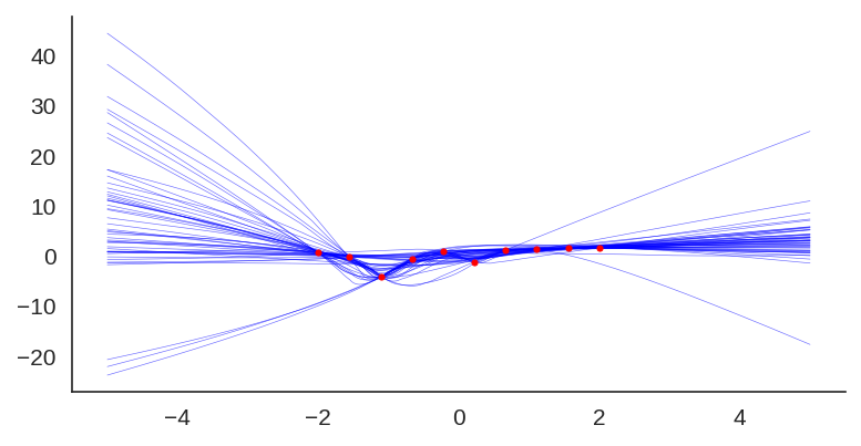
We can also visualize the individual model predictions showing their variability due to different initializations as well as the bootstrap noise:
Now, what is also quite interesting, is that we can change the prior to let’s say a fixed sine:
class SinPrior(nn.Module):
    def forward(self, input):
        return torch.sin(3 * input)
Then, when we train the same MLP model but this time using the sine prior, we can see how it affects the final prediction and uncertainty bounds:
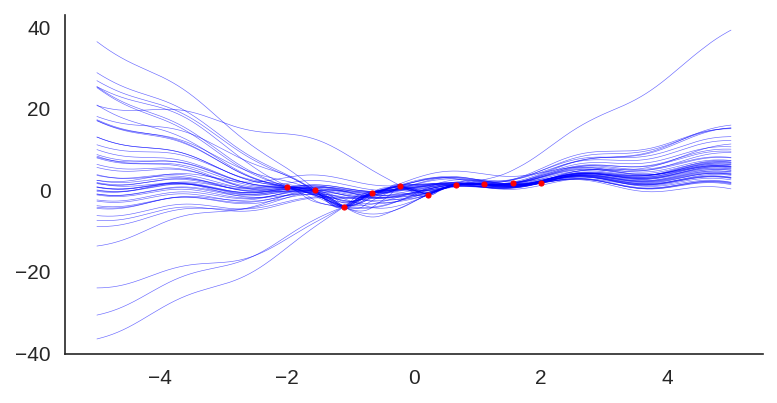
If we show each individual model, we can see the effect of the prior contribution to each individual model:
I hope you liked, these are quite amazing results for a simple method that at least pass the linear “sanity check”. I’ll explore some pre-trained networks in place of the prior to see the different effects on predictions, it’s a very interesting way to add some simple priors.

Hi, thanks for making the article. Can you post a link to the full source code – I’m still learning pytorch and struggling to get the code to work
Yeah I agree with Joe, would be amazing if you could publish the whole source code. 🙂
Either on the blog or as a repo on Github!
Best regards,
Phil