Year: 2019

Machine Learning

Uncertainty Estimation in Deep Learning (PyData Lisbon / July 2019)

Just sharing some slides I presented at the PyData Lisbon on July 2019 about the talk “Uncertainty Estimation in Deep Learning“:

Cite this article as: Christian S. Perone, "Uncertainty Estimation in Deep Learning (PyData Lisbon / July 2019)," in Terra Incognita, 18/07/2019, https://blog.christianperone.com/2019/07/uncertainty-estimation-in-deep-learning-pydata-lisbon-july-2019/.
Machine Learning

PyData Montreal slides for the talk: PyTorch under the hood

These are the slides of the talk I presented on PyData Montreal on Feb 25th. It was a pleasure to meet you all ! Thanks a lot to Maria and Alexander for the invitation !

Cite this article as: Christian S. Perone, "PyData Montreal slides for the talk: PyTorch under the hood," in Terra Incognita, 26/02/2019, https://blog.christianperone.com/2019/02/pydata-montreal-slides-for-the-talk-pytorch-under-the-hood/.
Machine Learning, Python

Listening to the neural network gradient norms during training

Training neural networks is often done by measuring many different metrics such as accuracy, loss, gradients, etc. This is most of the time done aggregating these metrics and plotting visualizations on TensorBoard.

There are, however, other senses that we can use to monitor the training of neural networks, such as sound. Sound is one of the perspectives that is currently very poorly explored in the training of neural networks. Human hearing can be very good a distinguishing very small perturbations in characteristics such as rhythm and pitch, even when these perturbations are very short in time or subtle.

For this experiment, I made a very simple example showing a synthesized sound that was made using the gradient norm of each layer and for step of the training for a convolutional neural network training on MNIST using different settings such as different learning rates, optimizers, momentum, etc.

You’ll need to install PyAudio and PyTorch to run the code (in the end of this post).

Training sound with SGD using LR 0.01

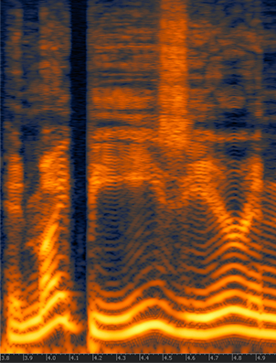
This segment represents a training session with gradients from 4 layers during the first 200 steps of the first epoch and using a batch size of 10. The higher the pitch, the higher the norm for a layer, there is a short silence to indicate different batches. Note the gradient increasing during time.

Training sound with SGD using LR 0.1

Same as above, but with higher learning rate.

Training sound with SGD using LR 1.0

Same as above, but with high learning rate that makes the network to diverge, pay attention to the high pitch when the norms explode and then divergence.

Training sound with SGD using LR 1.0 and BS 256

Same setting but with a high learning rate of 1.0 and a batch size of 256. Note how the gradients explode and then there are NaNs causing the final sound.

Training sound with Adam using LR 0.01

This is using Adam in the same setting as the SGD.


Source code

For those who are interested, here is the entire source code I used to make the sound clips:

import pyaudio
import numpy as np
import wave

import torch
import torch.nn as nn
import torch.nn.functional as F
import torch.optim as optim
from torchvision import datasets, transforms


class Net(nn.Module):
    def __init__(self):
        super(Net, self).__init__()
        self.conv1 = nn.Conv2d(1, 20, 5, 1)
        self.conv2 = nn.Conv2d(20, 50, 5, 1)
        self.fc1 = nn.Linear(4*4*50, 500)
        self.fc2 = nn.Linear(500, 10)

        self.ordered_layers = [self.conv1,
                               self.conv2,
                               self.fc1,
                               self.fc2]

    def forward(self, x):
        x = F.relu(self.conv1(x))
        x = F.max_pool2d(x, 2, 2)
        x = F.relu(self.conv2(x))
        x = F.max_pool2d(x, 2, 2)
        x = x.view(-1, 4*4*50)
        x = F.relu(self.fc1(x))
        x = self.fc2(x)
        return F.log_softmax(x, dim=1)


def open_stream(fs):
    p = pyaudio.PyAudio()
    stream = p.open(format=pyaudio.paFloat32,
                    channels=1,
                    rate=fs,
                    output=True)
    return p, stream


def generate_tone(fs, freq, duration):
    npsin = np.sin(2 * np.pi * np.arange(fs*duration) * freq / fs)
    samples = npsin.astype(np.float32)
    return 0.1 * samples


def train(model, device, train_loader, optimizer, epoch):
    model.train()

    fs = 44100
    duration = 0.01
    f = 200.0
    p, stream = open_stream(fs)

    frames = []

    for batch_idx, (data, target) in enumerate(train_loader):
        data, target = data.to(device), target.to(device)
        optimizer.zero_grad()
        output = model(data)
        loss = F.nll_loss(output, target)
        loss.backward()

        norms = []
        for layer in model.ordered_layers:
            norm_grad = layer.weight.grad.norm()
            norms.append(norm_grad)

            tone = f + ((norm_grad.numpy()) * 100.0)
            tone = tone.astype(np.float32)
            samples = generate_tone(fs, tone, duration)

            frames.append(samples)

        silence = np.zeros(samples.shape[0] * 2,
                           dtype=np.float32)
        frames.append(silence)

        optimizer.step()

        # Just 200 steps per epoach
        if batch_idx == 200:
            break

    wf = wave.open("sgd_lr_1_0_bs256.wav", 'wb')
    wf.setnchannels(1)
    wf.setsampwidth(p.get_sample_size(pyaudio.paFloat32))
    wf.setframerate(fs)
    wf.writeframes(b''.join(frames))
    wf.close()

    stream.stop_stream()
    stream.close()
    p.terminate()


def run_main():
    device = torch.device("cpu")

    train_loader = torch.utils.data.DataLoader(
        datasets.MNIST('../data', train=True, download=True,
                       transform=transforms.Compose([
                           transforms.ToTensor(),
                           transforms.Normalize((0.1307,), (0.3081,))
                       ])),
        batch_size=256, shuffle=True)

    model = Net().to(device)
    optimizer = optim.SGD(model.parameters(), lr=0.01, momentum=0.5)

    for epoch in range(1, 2):
        train(model, device, train_loader, optimizer, epoch)


if __name__ == "__main__":
    run_main()
Cite this article as: Christian S. Perone, "Listening to the neural network gradient norms during training," in Terra Incognita, 04/08/2019, https://blog.christianperone.com/2019/08/listening-to-the-neural-network-gradient-norms-during-training/.
Uncategorized

Visualizing network ensembles with bootstrap and randomized priors

A few months ago I made a post about Randomized Prior Functions for Deep Reinforcement Learning, where I showed how to implement the training procedure in PyTorch and how to extract the model uncertainty from them.

Using the same code showed earlier, these animations below show the training of an ensemble of 40 models with 2-layer MLP and 20 hidden units in different settings. These visualizations are really nice to understand what are the convergence differences when using or not bootstrap or randomized priors.

Naive Ensemble

This is a training session without bootstrapping data or adding a randomized prior, it’s just a naive ensembling:

Ensemble with Randomized Prior

This is the ensemble but with the addition of the randomized prior (MLP with the same architecture, with random weights and fixed):

$$Q_{\theta_k}(x) = f_{\theta_k}(x) + p_k(x)$$

The final model \(Q_{\theta_k}(x)\) will be the k model of the ensemble that will fit the function \(f_{\theta_k}(x)\) with an untrained prior \(p_k(x)\):

Ensemble with Randomized Prior and Bootstrap

This is a ensemble with the randomized prior functions and data bootstrap:

Ensemble with a fixed prior and bootstrapping

This is an ensemble with a fixed prior (Sin) and bootstrapping:

Cite this article as: Christian S. Perone, "Visualizing network ensembles with bootstrap and randomized priors," in Terra Incognita, 20/07/2019, https://blog.christianperone.com/2019/07/visualizing-network-ensembles-with-bootstrap-and-randomized-priors/.
Python

Numpy dispatcher: when Numpy becomes a protocol for an ecosystem

Introduction

Not a lot of people working with the Python scientific ecosystem are aware of the NEP 18 (dispatch mechanism for NumPy’s high-level array functions). Given the importance of this protocol, I decided to write this short introduction to the new dispatcher that will certainly bring a lot of benefits for the Python scientific ecosystem.

If you used PyTorch, TensorFlow, Dask, etc, you certainly noticed the similarity of their API contracts with Numpy. And it’s not by accident, Numpy’s API is one of the most fundamental and widely-used APIs for scientific computing. Numpy is so pervasive, that it ceased to be only an API and it is becoming more a protocol or an API specification.

(more…)

Machine Learning

Benford law on GPT-2 language model

I wrote some months ago about how the Benford law emerges from language models, today I decided to evaluate the same method to check how the GPT-2 would behave with some sentences and it turns out that it seems that it is also capturing these power laws. You can find some plots with the examples below, the plots are showing the probability of the digit given a particular sentence such as “with a population size of”, showing the distribution of: $$P(\{1,2, \ldots, 9\} \vert \text{“with a population size of”})$$ for the GPT-2 medium model (345M):

Cite this article as: Christian S. Perone, "Benford law on GPT-2 language model," in Terra Incognita, 14/06/2019, https://blog.christianperone.com/2019/06/benford-law-on-gpt-2-language-model/.

Machine Learning, Python

Randomized prior functions in PyTorch

Trained MLP with 2 hidden layers and a sine prior.

I was experimenting with the approach described in “Randomized Prior Functions for Deep Reinforcement Learning” by Ian Osband et al. at NPS 2018, where they devised a very simple and practical method for uncertainty using bootstrap and randomized priors and decided to share the PyTorch code.

I really like bootstrap approaches, and in my opinion, they are usually the easiest methods to implement and provide very good posterior approximation with deep connections to Bayesian approaches, without having to deal with variational inference. They actually show in the paper that in the linear case, the method provides a Bayes posterior.

The main idea of the method is to have bootstrap to provide a non-parametric data perturbation together with randomized priors, which are nothing more than just random initialized networks.

$$Q_{\theta_k}(x) = f_{\theta_k}(x) + p_k(x)$$

The final model \(Q_{\theta_k}(x)\) will be the k model of the ensemble that will fit the function \(f_{\theta_k}(x)\) with an untrained prior \(p_k(x)\).

Let’s go to the code. The first class is a simple MLP with 2 hidden layers and Glorot initialization :

class MLP(nn.Module):
    def __init__(self):
        super().__init__()
        self.l1 = nn.Linear(1, 20)
        self.l2 = nn.Linear(20, 20)
        self.l3 = nn.Linear(20, 1)
        
        nn.init.xavier_uniform_(self.l1.weight)
        nn.init.xavier_uniform_(self.l2.weight)
        nn.init.xavier_uniform_(self.l3.weight)

    def forward(self, inputs):
        x = self.l1(inputs)
        x = nn.functional.selu(x)
        x = self.l2(x)
        x = nn.functional.selu(x)
        x = self.l3(x)
        return x

Then later we define a class that will take the model and the prior to produce the final model result:

class ModelWithPrior(nn.Module):
    def __init__(self,
                 base_model : nn.Module,
                 prior_model : nn.Module,
                 prior_scale : float = 1.0):
        super().__init__()
        self.base_model = base_model
        self.prior_model = prior_model
        self.prior_scale = prior_scale

    def forward(self, inputs):
        with torch.no_grad():
            prior_out = self.prior_model(inputs)
            prior_out = prior_out.detach()
        model_out = self.base_model(inputs)
        return model_out + (self.prior_scale * prior_out)

And it’s basically that ! As you can see, it’s a very simple method, in the second part we just created a custom forward() to avoid computing/accumulating gradients for the prior network and them summing (after scaling) it with the model prediction.

To train it, you just have to use different bootstraps for each ensemble model, like in the code below:

def train_model(x_train, y_train, base_model, prior_model):
    model = ModelWithPrior(base_model, prior_model, 1.0)
    loss_fn = nn.MSELoss()
    optimizer = torch.optim.Adam(model.parameters(), lr=0.05)
    
    for epoch in range(100):
        model.train()
        preds = model(x_train)
        loss = loss_fn(preds, y_train)

        optimizer.zero_grad()
        loss.backward()
        optimizer.step()
            
    return model

and using a sampler with replacement (bootstrap) as in:

dataset = TensorDataset(...)
bootstrap_sampler = RandomSampler(dataset, True, len(dataset))
train_dataloader = DataLoader(dataset,
                              batch_size=len(dataset),
                              sampler=bootstrap_sampler)

In this case, I used the same small dataset used in the original paper:

After training it with a simple MLP prior as well, the results for the uncertainty are shown below:

Trained model with an MLP prior, used an ensemble of 50 models.

If we look at just the priors, we will see the variation of the untrained networks:

We can also visualize the individual model predictions showing their variability due to different initializations as well as the bootstrap noise:

Plot showing each individual model prediction and true data in red.

Now, what is also quite interesting, is that we can change the prior to let’s say a fixed sine:

class SinPrior(nn.Module):
    def forward(self, input):
        return torch.sin(3 * input)

Then, when we train the same MLP model but this time using the sine prior, we can see how it affects the final prediction and uncertainty bounds:

If we show each individual model, we can see the effect of the prior contribution to each individual model:

Plot showing each individual model of the ensemble trained with a sine prior.

I hope you liked, these are quite amazing results for a simple method that at least pass the linear “sanity check”. I’ll explore some pre-trained networks in place of the prior to see the different effects on predictions, it’s a very interesting way to add some simple priors.

Cite this article as: Christian S. Perone, "Randomized prior functions in PyTorch," in Terra Incognita, 24/03/2019, https://blog.christianperone.com/2019/03/randomized-prior-functions-in-pytorch/.

I'm starting a new course "Machine Learning: Foundations and Engineering" for 2024.