Update 28 Feb 2019: I added a new blog post with a slide deck containing the presentation I did for PyData Montreal.
Introduction
This post is a tour around the PyTorch codebase, it is meant to be a guide for the architectural design of PyTorch and its internals. My main goal is to provide something useful for those who are interested in understanding what happens beyond the user-facing API and show something new beyond what was already covered in other tutorials.
Note: PyTorch build system uses code generation extensively so I won’t repeat here what was already described by others. If you’re interested in understanding how this works, please read the following tutorials:
Short intro to Python extension objects in C/C++
As you probably know, you can extend Python using C and C++ and develop what is called as “extension”. All the PyTorch heavy work is implemented in C/C++ instead of pure-Python. To define a new Python object type in C/C++, you define a structure like this one example below (which is the base for the autograd Variable class):
// Python object that backs torch.autograd.Variable
struct THPVariable {
    PyObject_HEAD
    torch::autograd::Variable cdata;
    PyObject* backward_hooks;
};
As you can see, there is a macro at the beginning of the definition, called PyObject_HEAD, this macro’s goal is the standardization of Python objects and will expand to another structure that contains a pointer to a type object (which defines initialization methods, allocators, etc) and also a field with a reference counter.
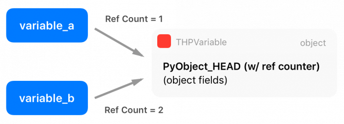
There are two extra macros in the Python API called Py_INCREF() and Py_DECREF(), which are used to increment and decrement the reference counter of Python objects. Multiple entities can borrow or own a reference to other objects (the reference counter is increased), and only when this reference counter reaches zero (when all references get destroyed), Python will automatically delete the memory from that object using its garbage collector.
You can read more about Python C/++ extensions here.
Funny fact: it is very common in many applications to use small integer numbers as indexing, counters, etc. For efficiency, the official
CPython interpreter caches the integers from -5 up to 256. For that reason, the statement
a = 200; b = 200; a is b will be
True, while the statement
a = 300; b = 300; a is b will be
False.
Zero-copy PyTorch Tensor to Numpy and vice-versa
PyTorch has its own Tensor representation, which decouples PyTorch internal representation from external representations. However, as it is very common, especially when data is loaded from a variety of sources, to have Numpy arrays everywhere, therefore we really need to make conversions between Numpy and PyTorch tensors. For that reason, PyTorch provides two methods called from_numpy() and numpy(), that converts a Numpy array to a PyTorch array and vice-versa, respectively. If we look the code that is being called to convert a Numpy array into a PyTorch tensor, we can get more insights on the PyTorch’s internal representation:
at::Tensor tensor_from_numpy(PyObject* obj) {
  if (!PyArray_Check(obj)) {
    throw TypeError("expected np.ndarray (got %s)", Py_TYPE(obj)->tp_name);
  }

  auto array = (PyArrayObject*)obj;
  int ndim = PyArray_NDIM(array);
  auto sizes = to_aten_shape(ndim, PyArray_DIMS(array));
  auto strides = to_aten_shape(ndim, PyArray_STRIDES(array));
  // NumPy strides use bytes. Torch strides use element counts.
  auto element_size_in_bytes = PyArray_ITEMSIZE(array);
  for (auto& stride : strides) {
    stride /= element_size_in_bytes;
  }

  // (...) - omitted for brevity

  void* data_ptr = PyArray_DATA(array);
  auto& type = CPU(dtype_to_aten(PyArray_TYPE(array)));
  Py_INCREF(obj);
  return type.tensorFromBlob(data_ptr, sizes, strides, [obj](void* data) {
    AutoGIL gil;
    Py_DECREF(obj);
  });
}
(code from tensor_numpy.cpp)
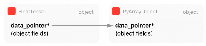
As you can see from this code, PyTorch is obtaining all information (array metadata) from Numpy representation and then creating its own. However, as you can note from the marked line 18, PyTorch is getting a pointer to the internal Numpy array raw data instead of copying it. This means that PyTorch will create a reference for this data, sharing the same memory region with the Numpy array object for the raw Tensor data.
There is also an important point here: when Numpy array object goes out of scope and get a zero reference count, it will be garbage collected and destroyed, that’s why there is an increment in the reference counting of the Numpy array object at line 20.
After this, PyTorch will create a new Tensor object from this Numpy data blob, and in the creation of this new Tensor it passes the borrowed memory data pointer, together with the memory size and strides as well as a function that will be used later by the Tensor Storage (we’ll discuss this in the next section) to release the data by decrementing the reference counting to the Numpy array object and let Python take care of this object life cycle.
The tensorFromBlob() method will create a new Tensor, but only after creating a new “Storage” for this Tensor. The storage is where the actual data pointer will be stored (and not in the Tensor structure itself). This takes us to the next section about Tensor Storages.
Tensor Storage
The actual raw data of the Tensor is not directly kept in the Tensor structure, but on another structure called Storage, which in turn is part of the Tensor structure.
As we saw in the previous code from tensor_from_numpy(), there is a call for tensorFromBlob() that will create a Tensor from the raw data blob. This last function will call another function called storageFromBlob() that will, in turn, create a storage for this data according to its type. In the case of a CPU float type, it will return a new CPUFloatStorage instance.
The CPUFloatStorage is basically a wrapper with utility functions around the actual storage structure called THFloatStorage that we show below:
typedef struct THStorage
{
    real *data;
    ptrdiff_t size;
    int refcount;
    char flag;
    THAllocator *allocator;
    void *allocatorContext;
    struct THStorage *view;
} THStorage;
(code from THStorage.h)
As you can see, the THStorage holds a pointer to the raw data, its size, flags and also an interesting field called allocator that we’ll soon discuss. It is also important to note that there is no metadata regarding on how to interpret the data inside the THStorage, this is due to the fact that the storage is “dumb” regarding of its contents and it is the Tensor responsibility to know how to “view” or interpret this data.
From this, you already probably realized that we can have multiple tensors pointing to the same storage but with different views of this data, and that’s why viewing a tensor with a different shape (but keeping the same number of elements) is so efficient. This Python code below shows that the data pointer in the storage is being shared after changing the way Tensor views its data:
>>> tensor_a = torch.ones((3, 3))
>>> tensor_b = tensor_a.view(9)
>>> tensor_a.storage().data_ptr() == tensor_b.storage().data_ptr()
True
As we can see in the example above, the data pointer on the storage of both Tensors are the same, but the Tensors represent a different interpretation of the storage data.
Now, as we saw in line 7 of the THFloatStorage structure, there is a pointer to a THAllocator structure there. And this is very important because it brings flexibility regarding the allocator that can be used to allocate the storage data. This structure is represented by the following code:
typedef struct THAllocator
{
  void* (*malloc)(void*, ptrdiff_t);
  void* (*realloc)(void*, void*, ptrdiff_t);
  void (*free)(void*, void*);
} THAllocator;
(code from THAllocator.h)
As you can see, there are three function pointer fields in this structure to define what an allocator means: a malloc, realloc and free. For CPU-allocated memory, these functions will, of course, relate to the traditional malloc/realloc/free POSIX functions, however, when we want a storage allocated on GPUs we’ll end up using the CUDA allocators such as the cudaMallocHost(), like we can see in the THCudaHostAllocator malloc function below:
static void *THCudaHostAllocator_malloc(void* ctx, ptrdiff_t size) {
  void* ptr;
  if (size < 0) THError("Invalid memory size: %ld", size);
  if (size == 0) return NULL;
  THCudaCheck(cudaMallocHost(&ptr, size));
  return ptr;
}
(code from THCAllocator.c)
You probably noticed a pattern in the repository organization, but it is important to keep in mind these conventions when navigating the repository, as summarized here (taken from the PyTorch lib readme):
- TH = TorcH
- THC = TorcH Cuda
- THCS = TorcH Cuda Sparse
- THCUNN = TorcH CUda Neural Network
- THD = TorcH Distributed
- THNN = TorcH Neural Network
- THS = TorcH Sparse
This convention is also present in the function/class names and other objects, so it is important to always keep these patterns in mind. While you can find CPU allocators in the TH code, you’ll find CUDA allocators in the THC code.
Finally, we can see the composition of the main Tensor THTensor structure:
typedef struct THTensor
{
    int64_t *size;
    int64_t *stride;
    int nDimension;
    THStorage *storage;
    ptrdiff_t storageOffset;
    int refcount;
    char flag;
} THTensor;
(Code from THTensor.h)
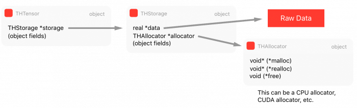
And as you can see, the main THTensor structure holds the size/strides/dimensions/offsets/etc as well as the storage (THStorage) for the Tensor data.
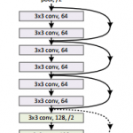
We can summarize all this structure that we saw in the diagram below:
Now, once we have requirements such as multi-processing where we want to share tensor data among multiple different processes, we need a shared memory approach to solve it, otherwise, every time another process needs a tensor or even when you want to implement Hogwild training procedure where all different processes will write to the same memory region (where the parameters are), you’ll need to make copies between processes, and this is very inefficient. Therefore we’ll discuss in the next section a special kind of storage for Shared Memory.
Shared Memory
Shared memory can be implemented in many different ways depending on the platform support. PyTorch supports some of them, but for the sake of simplicity, I’ll talk here about what happens on MacOS using the CPU (instead of GPU). Since PyTorch supports multiple shared memory approaches, this part is a little tricky to grasp into since it involves more levels of indirection in the code.
PyTorch provides a wrapper around the Python multiprocessing module and can be imported from torch.multiprocessing. The changes they implemented in this wrapper around the official Python multiprocessing were done to make sure that everytime a tensor is put on a queue or shared with another process, PyTorch will make sure that only a handle for the shared memory will be shared instead of a new entire copy of the Tensor.
Now, many people aren’t aware of a Tensor method from PyTorch called share_memory_(), however, this function is what triggers an entire rebuild of the storage memory for that particular Tensor. What this method does is to create a region of shared memory that can be used among different processes. This function will, in the end, call this following function below:
static THStorage* THPStorage_(newFilenameStorage)(ptrdiff_t size)
{
  int flags = TH_ALLOCATOR_MAPPED_SHAREDMEM | TH_ALLOCATOR_MAPPED_EXCLUSIVE;
  std::string handle = THPStorage_(__newHandle)();
  auto ctx = libshm_context_new(NULL, handle.c_str(), flags);
  return THStorage_(newWithAllocator)(size, &THManagedSharedAllocator, (void*)ctx);
}
(Code from StorageSharing.cpp)
And as you can see, this function will create another storage using a special allocator called THManagedSharedAllocator. This function first defines some flags and then it creates a handle which is a string in the format /torch_[process id]_[random number], and after that, it will then create a new storage using the special THManagedSharedAllocator. This allocator has function pointers to an internal PyTorch library called libshm, that will implement a Unix Domain Socket communication to share the shared memory region handles. This allocator is actual an especial case and it is a kind of “smart allocator” because it contains the communication control logic as well as it uses another allocator called THRefcountedMapAllocator that will be responsible for creating the actual shared memory region and call mmap() to map this region to the process virtual address space.
Note: when a method ends with a underscore in PyTorch, such as the method called share_memory_(), it means that this method has an in-place effect, and it will change the current object instead of creating a new one with the modifications.
I’ll now show a Python example of one processing using the data from a Tensor that was allocated on another process by manually exchanging the shared memory handle:
This is executed in the process A:
>>> import torch
>>> tensor_a = torch.ones((5, 5))
>>> tensor_a

 1  1  1  1  1
 1  1  1  1  1
 1  1  1  1  1
 1  1  1  1  1
 1  1  1  1  1
[torch.FloatTensor of size 5x5]

>>> tensor_a.is_shared()
False
>>> tensor_a = tensor_a.share_memory_()
>>> tensor_a.is_shared()
True
>>> tensor_a_storage = tensor_a.storage()
>>> tensor_a_storage._share_filename_()
(b'/var/tmp/tmp.0.yowqlr', b'/torch_31258_1218748506', 25)
In this code, executed in the process A, we create a new Tensor of 5×5 filled with ones. After that we make it shared and print the tuple with the Unix Domain Socket address as well as the handle. Now we can access this memory region from another process B as shown below:
Code executed in the process B:
>>> import torch
>>> tensor_a = torch.Tensor()
>>> tuple_info = (b'/var/tmp/tmp.0.yowqlr', b'/torch_31258_1218748506', 25)
>>> storage = torch.Storage._new_shared_filename(*tuple_info)
>>> tensor_a = torch.Tensor(storage).view((5, 5))

 1  1  1  1  1
 1  1  1  1  1
 1  1  1  1  1
 1  1  1  1  1
 1  1  1  1  1
[torch.FloatTensor of size 5x5]
As you can see, using the tuple information about the Unix Domain Socket address and the handle we were able to access the Tensor storage from another process. If you change the tensor in this process B, you’ll also see that it will reflect in the process A because these Tensors are sharing the same memory region.
DLPack: a hope for the Deep Learning frameworks Babel
Now I would like to talk about something recent in the PyTorch code base, that is called DLPack. DLPack is an open standardization of an in-memory tensor structure that will allow exchange tensor data between frameworks, and what is quite interesting is that since this memory representation is standardized and very similar to the memory representation already in use by many frameworks, it will allow a zero-copy data sharing between frameworks, which is a quite amazing initiative given the variety of frameworks we have today without inter-communication among them.
This will certainly help to overcome the “island model” that we have today between tensor representations in MXNet, PyTorch, etc, and will allow developers to mix framework operations between frameworks and all the benefits that a standardization can bring to the frameworks.
The core of DLPack os a very simple structure called DLTensor, as shown below:
/*!
 * \brief Plain C Tensor object, does not manage memory.
 */
typedef struct {
  /*!
   * \brief The opaque data pointer points to the allocated data.
   *  This will be CUDA device pointer or cl_mem handle in OpenCL.
   *  This pointer is always aligns to 256 bytes as in CUDA.
   */
  void* data;
  /*! \brief The device context of the tensor */
  DLContext ctx;
  /*! \brief Number of dimensions */
  int ndim;
  /*! \brief The data type of the pointer*/
  DLDataType dtype;
  /*! \brief The shape of the tensor */
  int64_t* shape;
  /*!
   * \brief strides of the tensor,
   *  can be NULL, indicating tensor is compact.
   */
  int64_t* strides;
  /*! \brief The offset in bytes to the beginning pointer to data */
  uint64_t byte_offset;
} DLTensor;
(code from dlpack.h)
As you can see, there is a data pointer for the raw data as well as shape/stride/offset/GPU vs CPU, and other metadata information about the data that the DLTensor pointing to.
There is also a managed version of the tensor that is called DLManagedTensor, where the frameworks can provide a context and also a “deleter” function that can be called by the framework who borrowed the Tensor to inform the other framework that the resources are no longer required.
In PyTorch, if you want to convert to or from a DLTensor format, you can find both C/C++ methods for doing that or even in Python you can do that as shown below:
import torch
from torch.utils import dlpack

t = torch.ones((5, 5))
dl = dlpack.to_dlpack(t)
This Python function will call the toDLPack function from ATen, shown below:
DLManagedTensor* toDLPack(const Tensor& src) {
  ATenDLMTensor * atDLMTensor(new ATenDLMTensor);
  atDLMTensor->handle = src;
  atDLMTensor->tensor.manager_ctx = atDLMTensor;
  atDLMTensor->tensor.deleter = &deleter;
  atDLMTensor->tensor.dl_tensor.data = src.data_ptr();
  int64_t device_id = 0;
  if (src.type().is_cuda()) {
    device_id = src.get_device();
  }
  atDLMTensor->tensor.dl_tensor.ctx = getDLContext(src.type(), device_id);
  atDLMTensor->tensor.dl_tensor.ndim = src.dim();
  atDLMTensor->tensor.dl_tensor.dtype = getDLDataType(src.type());
  atDLMTensor->tensor.dl_tensor.shape = const_cast<int64_t*>(src.sizes().data());
  atDLMTensor->tensor.dl_tensor.strides = const_cast<int64_t*>(src.strides().data());
  atDLMTensor->tensor.dl_tensor.byte_offset = 0;
  return &(atDLMTensor->tensor);
}
As you can see, it’s a pretty simple conversion, casting the metadata from the PyTorch format to the DLPack format and assigning a pointer to the internal Tensor data representation.
I really hope that more frameworks adopt this standard that will certainly give benefits to the ecosystem. It is also interesting to note that a potential integration with Apache Arrow would be amazing.
That’s it, I hope you liked this long post !
– Christian S. Perone


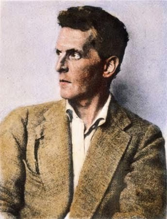 One of the most interesting aspects of Wittgenstein is perhaps that fact that he had developed two very different philosophies during his life, and each of which had great influence. Something quite rare for someone who spent so much time working on these ideas and retreating even after the major influence they exerted, especially in the Vienna Circle. A true lesson of intellectual honesty, and in my opinion, one important legacy.
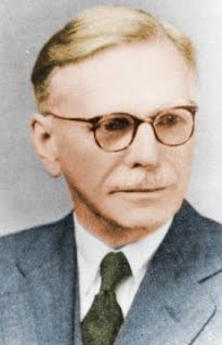 John R. Firth