2013 | Terra Incognita

Bitcoin, Programming, Python

The beauty of Bitcoin P2P network

So, in the last days I just released Protocoin, a framework in pure Python with a Bitcoin P2P network implementation. While I’m in process of development of the v.0.2 of the framework (with new and nice features like Bitcoin keys management – you can see some preview here) I would like to show a real-time visualization I’ve made with Protocoin and Ubigraph of a node connecting to a seed node and then issuing GetAddr message for each node and connecting on the received nodes in a breadth-first search fashion. I’ll release the code used to create this visualization in the next release of Protocoin as soon as possible. I hope you enjoy it !

Color legend

Yellow = Connecting
Green = Connected
Blue = Disconnected after connection

Video

13/12/2013 by Christian S. Perone

Programming, Python

Protocoin – a pure Python Bitcoin protocol implementation

Just release the first version of Protocoin, a pure Python Bitcoin protocol implementation, for more information see the documentation or the project in Github.

If you want to donate for the project, my Bitcoin address is: 1Q6JZEE5turJXaTn1fburWkqjhC4oMJ4yV.

I hope you like it !

– Christian S. Perone

22/11/2013 by Christian S. Perone

Programming, Python

Mapa de calor dos dados de acidentes de transito do DataPoa

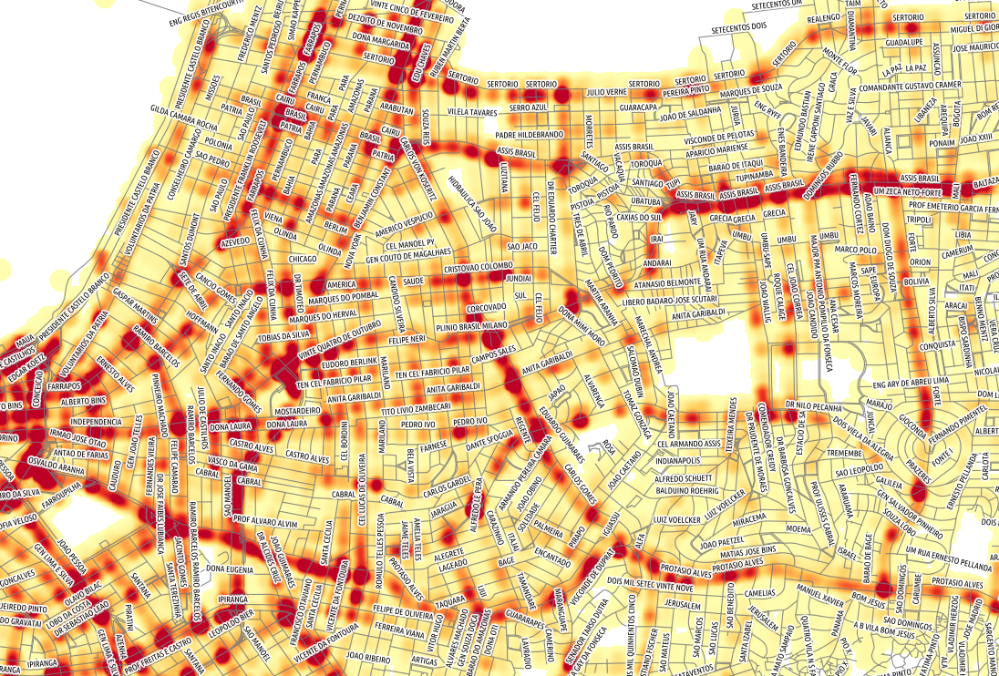
Esta semana será disponibilzada a nova versão do Django GIS Brasil, segue abaixo um exemplo de mapa criado usando os novos dados do Django GIS Brasil importados do DataPoa.

O exemplo abaixo é um mapa de calor utilizando os dados de acidentes de trânsito em Porto Alegre /RS durante os anos de 2000 até 2012. Os eixos (ruas, avenidas, etc.) também estarão presentes no Django GIS Brasil.

Heatmap POA — Mapa de Acidentes de Trânsito em PoA/RS. Clique para ampliar.

16/11/2013 by Christian S. Perone

Uncategorized

Book Suggestion: Codex Seraphinianus

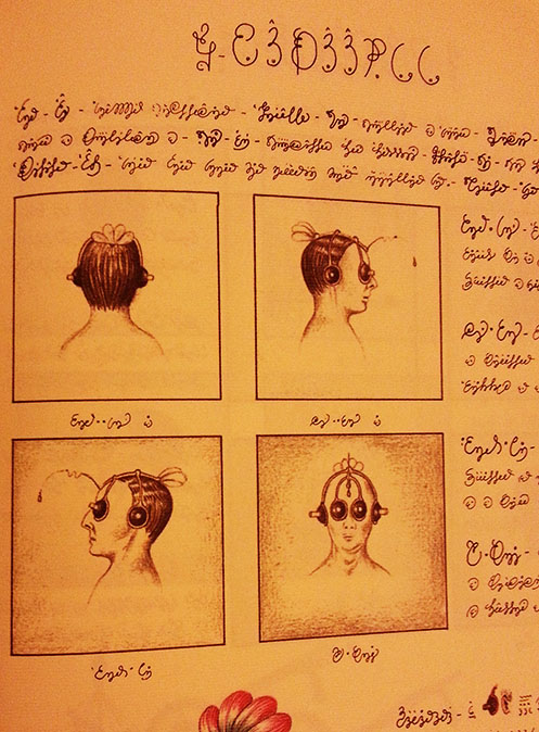
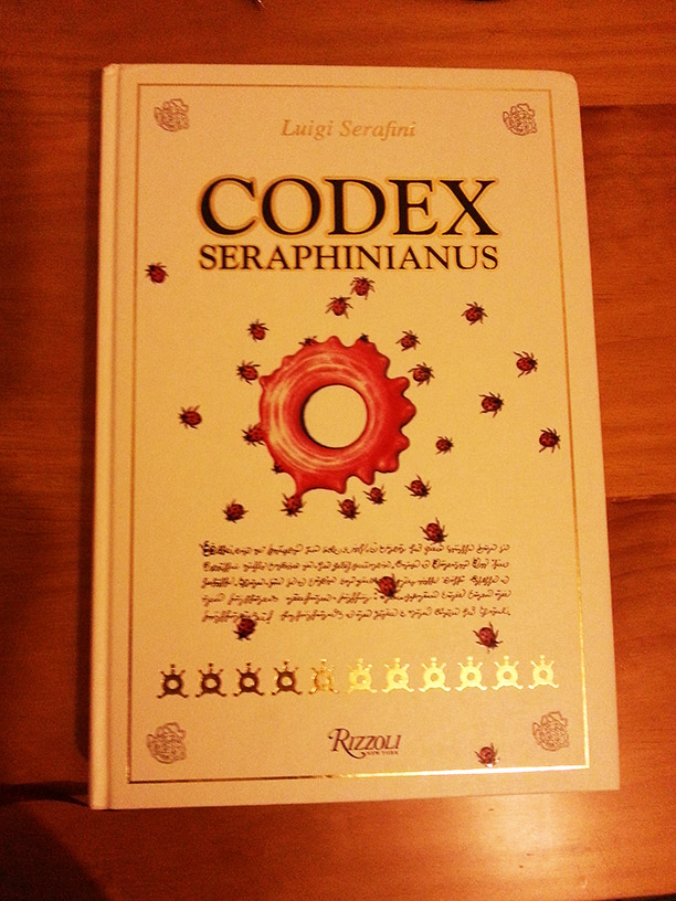
Today the Codex Seraphinianus just arrived (after months waiting in the pre-order state). I bought it from Amazon and I really recommend this edition for those who are interested because this is a very large edition with high quality textured paper and beautiful printing style. The book has also in the end a pocket with a small brochure called “Decodex” with a letter from Luigi Serafini.

The book is a very impressive creation by Luigi Serafini (or by the cat) dating from 1981 and presenting an impossible world that will cause to you the most strange feelings. See the photo of the cover and some pages below.

– Christian S. Perone

05/11/2013 by Christian S. Perone

Machine Learning, Programming, Python

Machine Learning :: Cosine Similarity for Vector Space Models (Part III)

* It has been a long time since I wrote the TF-IDF tutorial (Part I and Part II) and as I promissed, here is the continuation of the tutorial. Unfortunately I had no time to fix the previous tutorials for the newer versions of the scikit-learn (sklearn) package nor to answer all the questions, but I hope to do that in a close future.

So, on the previous tutorials we learned how a document can be modeled in the Vector Space, how the TF-IDF transformation works and how the TF-IDF is calculated, now what we are going to learn is how to use a well-known similarity measure (Cosine Similarity) to calculate the similarity between different documents.

The Dot Product

Let’s begin with the definition of the dot product for two vectors: $\vec{a} = (a_1, a_2, a_3, \ldots)$ and $\vec{b} = (b_1, b_2, b_3, \ldots)$ , where $a_n$ and $b_n$ are the components of the vector (features of the document, or TF-IDF values for each word of the document in our example) and the $\mathit{n}$ is the dimension of the vectors:

$\vec{a} \cdot \vec{b} = \sum_{i=1}^n a_ib_i = a_1b_1 + a_2b_2 + \cdots + a_nb_n$

As you can see, the definition of the dot product is a simple multiplication of each component from the both vectors added together. See an example of a dot product for two vectors with 2 dimensions each (2D):

$\vec{a} = (0, 3) \\ \vec{b} = (4, 0) \\ \vec{a} \cdot \vec{b} = 0*4 + 3*0 = 0$

The first thing you probably noticed is that the result of a dot product between two vectors isn’t another vector but a single value, a scalar.

This is all very simple and easy to understand, but what is a dot product ? What is the intuitive idea behind it ? What does it mean to have a dot product of zero ? To understand it, we need to understand what is the geometric definition of the dot product:

$\vec{a} \cdot \vec{b} = \|\vec{a}\|\|\vec{b}\|\cos{\theta}$

Rearranging the equation to understand it better using the commutative property, we have:

$\vec{a} \cdot \vec{b} = \|\vec{b}\|\|\vec{a}\|\cos{\theta}$

So, what is the term $\displaystyle \|\vec{a}\|\cos{\theta}$ ? This term is the projection of the vector $\vec{a}$ into the vector $\vec{b}$ as shown on the image below:

Dot_Product — The projection of the vector A into the vector B. By Wikipedia.

Now, what happens when the vector $\vec{a}$ is orthogonal (with an angle of 90 degrees) to the vector $\vec{b}$ like on the image below ?

vectors1 — Two orthogonal vectors (with 90 degrees angle).

There will be no adjacent side on the triangle, it will be equivalent to zero, the term $\displaystyle \|\vec{a}\|\cos{\theta}$ will be zero and the resulting multiplication with the magnitude of the vector $\vec{b}$ will also be zero. Now you know that, when the dot product between two different vectors is zero, they are orthogonal to each other (they have an angle of 90 degrees), this is a very neat way to check the orthogonality of different vectors. It is also important to note that we are using 2D examples, but the most amazing fact about it is that we can also calculate angles and similarity between vectors in higher dimensional spaces, and that is why math let us see far than the obvious even when we can’t visualize or imagine what is the angle between two vectors with twelve dimensions for instance.

The Cosine Similarity

The cosine similarity between two vectors (or two documents on the Vector Space) is a measure that calculates the cosine of the angle between them. This metric is a measurement of orientation and not magnitude, it can be seen as a comparison between documents on a normalized space because we’re not taking into the consideration only the magnitude of each word count (tf-idf) of each document, but the angle between the documents. What we have to do to build the cosine similarity equation is to solve the equation of the dot product for the $\cos{\theta}$ :

$\displaystyle \vec{a} \cdot \vec{b} = \|\vec{a}\|\|\vec{b}\|\cos{\theta} \\ \\ \cos{\theta} = \frac{\vec{a} \cdot \vec{b}}{\|\vec{a}\|\|\vec{b}\|}$

And that is it, this is the cosine similarity formula. Cosine Similarity will generate a metric that says how related are two documents by looking at the angle instead of magnitude, like in the examples below:

cosinesimilarityfq1 — The Cosine Similarity values for different documents, 1 (same direction), 0 (90 deg.), -1 (opposite directions).

Note that even if we had a vector pointing to a point far from another vector, they still could have an small angle and that is the central point on the use of Cosine Similarity, the measurement tends to ignore the higher term count on documents. Suppose we have a document with the word “sky” appearing 200 times and another document with the word “sky” appearing 50, the Euclidean distance between them will be higher but the angle will still be small because they are pointing to the same direction, which is what matters when we are comparing documents.

Now that we have a Vector Space Model of documents (like on the image below) modeled as vectors (with TF-IDF counts) and also have a formula to calculate the similarity between different documents in this space, let’s see now how we do it in practice using scikit-learn (sklearn).

Practice Using Scikit-learn (sklearn)

* In this tutorial I’m using the Python 2.7.5 and Scikit-learn 0.14.1.

The first thing we need to do is to define our set of example documents:

documents = (
"The sky is blue",
"The sun is bright",
"The sun in the sky is bright",
"We can see the shining sun, the bright sun"
)

And then we instantiate the Sklearn TF-IDF Vectorizer and transform our documents into the TF-IDF matrix:

from sklearn.feature_extraction.text import TfidfVectorizer
tfidf_vectorizer = TfidfVectorizer()
tfidf_matrix = tfidf_vectorizer.fit_transform(documents)
print tfidf_matrix.shape
(4, 11)

Now we have the TF-IDF matrix (tfidf_matrix) for each document (the number of rows of the matrix) with 11 tf-idf terms (the number of columns from the matrix), we can calculate the Cosine Similarity between the first document (“The sky is blue”) with each of the other documents of the set:

from sklearn.metrics.pairwise import cosine_similarity
cosine_similarity(tfidf_matrix[0:1], tfidf_matrix)
array([[ 1.        ,  0.36651513,  0.52305744,  0.13448867]])

The tfidf_matrix[0:1] is the Scipy operation to get the first row of the sparse matrix and the resulting array is the Cosine Similarity between the first document with all documents in the set. Note that the first value of the array is 1.0 because it is the Cosine Similarity between the first document with itself. Also note that due to the presence of similar words on the third document (“The sun in the sky is bright”), it achieved a better score.

If you want, you can also solve the Cosine Similarity for the angle between vectors:

$\cos{\theta} = \frac{\vec{a} \cdot \vec{b}}{\|\vec{a}\|\|\vec{b}\|}$

We only need to isolate the angle ( $\theta$ ) and move the $\cos$ to the right hand of the equation:

$\theta = \arccos{\frac{\vec{a} \cdot \vec{b}}{\|\vec{a}\|\|\vec{b}\|}}$

The $\arccos$ is the same as the inverse of the cosine ( $\cos^-1$ ).

Lets for instance, check the angle between the first and third documents:

import math
# This was already calculated on the previous step, so we just use the value
cos_sim = 0.52305744
angle_in_radians = math.acos(cos_sim)
print math.degrees(angle_in_radians)
58.462437107432784

And that angle of ~58.5 is the angle between the first and the third document of our document set.

That is it, I hope you liked this third tutorial !

Cite this article as: Christian S. Perone, "Machine Learning :: Cosine Similarity for Vector Space Models (Part III)," in Terra Incognita, 12/09/2013, https://blog.christianperone.com/2013/09/machine-learning-cosine-similarity-for-vector-space-models-part-iii/.

Related Material

A video about Dot Product on The Khan Academy

Wikipedia: Dot Product

Wikipedia: Cosine Similarity

Scikit-learn (sklearn) – The de facto Machine Learning package for Python

12/09/201319/01/2020 by Christian S. Perone

Raspberry Pi

Rastreamento em tempo real de avioes em Porto Alegre utilizando Raspberry Pi + Radio UHF (SDR RTL2832U)

* This post is in Portuguese.

SDR (Software-Defined Radio)

SDR é uma área de radiocomunicação baseada em uma ideia muito simples: implementar em software o que antes era implementado em hardware (ex: mod/demod, filtros, etc). O fato do SDR estar se tornando uma tendência hoje se dá principalmente pelo baixo custo de alguns receptores como por exemplo o RTL2832U (mais sobre ele depois) que hoje você pode encontrar facilmente por uns U$ 20.00, preço este muito barato se você levar em consideração o intervalo de cobertura das frequências de 22Mhz até 2200Mhz (dependendo do tuner). Neste intervalo dá pra se ter uma ampla cobertura de sinais de rádio AM/FM, rádio da polícia, TV, GSM, GPS, ADSB (este post é sobre o ADSB), comunicação marítma, LTE (ainda em definição no Brasil) e outras aplicações que estão inseridas neste intervalo de frequência.

Um sistema SDR é composto geralmente por: um receptor ligado ao computador ou qualquer outro dispositivo embarcado com um poder de processamento razoável (por meio de placa de captura de áudio, USB, etc) e um software que irá fazer o tratamento do sinal recebido. Neste post eu vou utilizar o Raspberry Pi como dispositivo embarcado para capturar e demodular os dados enviados pelos transponders presentes em aeronaves comerciais e domésticas.

ADS-B (Automatic dependent surveillance-broadcast)

Grande parte dos aviões modernos estão sendo equipados com um dispositivo que tem o objetivo de substituir os radares que existem hoje. Até o ano de 2020 todos os aviões que entrarem no espaço aéreo estadunidense deverão ter como item obrigatório um dispositivo compatível com ADS-B. O dispositivo ADS-B faz com que as aeronaves sejam visíveis aos radares em terra e também para outros aviões através do broadcast de mensagens com sua altura, velocidade, posição e muitas outras informações relevantes. A transmissão destas mensagens se dá através da frequência 1090Mhz, uma frequência dentro do intervalo de captura de maioria dos receptores SDR usando o chipset RTL2832U. A ideia deste post é usar o Raspberry Pi para receber este broadcast enviado diretamente pelo transponder dos aviões, demodular os frames e então utilizar um software para decodificar/interpretar os frames e plotar em um mapa a posição atual dos aviões em Porto Alegre / RS.

Realtek RTL2832U

Alguns receptores de TV digital USB utilizam o chipset da Realtek RTL2832U, como este meu acima. Em 2012 foi descoberto que este chipset permitia o envio de dados brutos do receptor para o host, permitindo assim seu uso para SDR. Existem alguns projetos com drivers para se comunicar com o dispositivo e receber estes dados (Linux e Windows), entre os quais o mais utilizado em Linux é o projeto rtl-sdr, que agrega além do driver alguns utilitários de linha de comando como por exemplo o “rtl_adsb” que utilizarei no Raspberry Pi para demodular o sinal ADS-B enviado pelas aeronaves; outro componente importante nos receptores USB é o tuner, que é responsável pelo ajuste da frequencia do rádio, no caso do meu dongle USB ele é o R820T que tem uma ótima sensibilidade mas tem um intervalo menor de cobertura do espectro quando comparado ao E4000 (da Elonics), veja a tabela no site do projeto para saber o intervalo de cobertura de cada tuner e de outros hardwares suportados pelo rtl-sdr.

Compilando o rtl-sdr no Raspberry Pi

Estou utilizando o Raspberry Pi como host do dongle USB porque ele é um aparelho barato e o consumo de energia é muito baixo, ou seja, você pode deixá-lo ligado capturando o sinal ADS-B por quanto tempo quiser sem se preocupar com um gasto maior que 5 watts no pior caso.

Baixando repositório

git clone git://git.osmocom.org/rtl-sdr.git

Dependências: libusb-1.0-0-dev, cmake, compilador (gcc)

Criando arquivos para compilação e compilando:

cd rtl-sdr/
mkdir build
cd build
cmake ../
make
sudo make install
sudo ldconfig

E pronto, já estamos com o rtl-sdr instalado (driver a aplicativos extras).

Recebendo sinal ADS-B

Antes de mais nada, um pequeno teste para verificar se o rtl-sdr está encontrando corretamente o dongle USB:

pi@raspberrypi ~ $ rtl_test -t
Found 1 device(s):
0: ezcap USB 2.0 DVB-T/DAB/FM dongle

Using device 0: ezcap USB 2.0 DVB-T/DAB/FM dongle

Found Rafael Micro R820T tuner

Supported gain values (29): 0.0 0.9 1.4 2.7 3.7 7.7

8.7 12.5 14.4 15.7 16.6 19.7 20.7 22.9 25.4 28.0

29.7 32.8 33.8 36.4 37.2 38.6 40.2 42.1 43.4 43.9

44.5 48.0 49.6

No E4000 tuner found, aborting.

pi@raspberrypi ~ $

Note que o meu dongle é um RTL2832U com o tuner R820T, ao executar o “rtl_test -t” é também exibida uma lista com os ganhos suportados pelo dongle.

Como a frequência utilizada pelo ADS-B é de 1090MHz, uma antena boa seria uma discone ou uma dipolo confeccionada com as dimensões corretas para esta frequência. Como ainda não tenho os plugs adequados tive que utiliar a antena que veio junto com o dongle, que mesmo sendo de baixa qualidade e não relacionada com a frequência do ADS-B ainda consegue receber os sinais (de fato, mesmo desconectando a antena eu consigo receber os frames das aeronaves), mesmo com o dongle em um ambiente fechado (minha casa fica há uns 6-10km do aeroporto de Porto Alegre / RS).

Para receber e demodular os frames eu utilizei o utilitário “rtl_adsb” (ele vem junto com o pacote do rtl-sdr). Ao ser executado, ele ajustará o tuner para a frequência do transponder das aeronaves em 1090MHz e logo após fará a demodulação dos frames para o formato hexadecimal:

pi@raspberrypi ~ $ rtl_adsb
Found 1 device(s):
0: Realtek, RTL2838UHIDIR, SN: 00000013

Using device 0: ezcap USB 2.0 DVB-T/DAB/FM dongle
Found Rafael Micro R820T tuner
Tuner gain set to automatic.
Tuned to 1090000000 Hz.
Sampling at 2000000 Hz.
Exact sample rate is: 2000000.052982 Hz
*825566cf477b3124c64b17e74b15;
*e6c7d7fdb34c855db6972204ea14;
*d1e27bb95df2454ca547c87718a2;
*906bc5a59b5c5053226fb94f3460;
*a6f51dc76353efeeabfbfe6946cb;
*e78ed3aaf547fcd87e8e4f41cea3;
*d26a5ecacdb7051f2ebe18efc613;

Cada frame inicia sempre com um asterisco na frente e cada um destes frames foi enviado diretamente por um transponder de um avião ou é uma requisição terra->ar de alguma base em terra. O que precisamos agora é fazer a decodificação destes frames para poder extrair o tipo do frame, latitude, longitude, callsign, origem e destino do avião, etc. Não existem hoje muitas alternativas open-source para fazer o plot dos aviões em um mapa, o melhor que eu encontrei foi o Virtual Radar Server que é open-source e roda também em Linux, além de ter uma interface web bem amigável e plotar as aeronaves usando o Google Maps.
Para fazer com que o Virtual Radar Server conecte no Raspberry Pi, primeiramente precisamos fazer o streaming via TCP dos frames que o “rtl_adsb” está recebendo no Raspberry Pi, o que dá para resolver utilizando o “netcat” mesmo:

rtl_adsb | netcat -lp 8080

Neste caso ele irá escutar na porta 8080 e enviar os frames ADS-B para o cliente que conectar nele. Logo após é só especificar o IP/porta do Raspberry Pi no Virtual Radar Server e se tudo der certo e você conseguir receber algum frame de algum transponder, você verá uma tela parecida com esta mostrada abaixo com o rastreamento dos aviões em tempo real:

No screenshot você pode ver um avião da GOL (GOL1446) se dirigindo ao aeroporto (logo a frente onde diz São João) a uma velocidade de 250km/h e descendo a uma velocidade de 195 metros por minuto. Geralmente os aviões enviam o broadcast da mensagem com a posição a cada segundo, tudo vai depender da sua antena, receptor e condições de difusão. Com a minha antena pequena e no meio de prédios eu consegui capturar o broadcast de aviõe em até uns 80km de distância, espero melhorar isto com uma outra antena, só preciso achar o material agora =)