Credit: ESA/Webb, NASA & CSA, J. Rigby. / The James Webb Space Telescope captures gravitational lensing, a phenomenon that can be modeled using differential geometry.
Note: This is a continuation of the previous post: Thoughts on Riemannian metrics and its connection with diffusion/score matching [Part I], so if you haven’t read it yet, please consider reading as I won’t be re-introducing in depth the concepts (e.g., the two scores) that I described there already. This article became a bit long, so if you are familiar already with metric tensors and differential geometry you can just skip the first part.
I was planning to write a paper about this topic, but my spare time is not that great so I decided it would be much more fun and educative to write this article in form of a tutorial. If you liked it, please consider citing it:
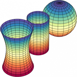
Different gaussian curvature surfaces. Image by Nicoguaro.
We are so used to Euclidean geometry that we often overlook the significance of curved geometries and the methods for measuring things that don’t reside on orthonormal bases. Just as understanding physics and the curvature of spacetime requires Riemannian geometry, I believe a profound comprehension of Machine Learning (ML) and data is also not possible without it. There is an increasing body of research that integrates differential geometry into ML. Unfortunately, the term “geometric deep learning” has predominantly become associated with graphs. However, modern geometry offers much more than just graph-related applications in ML.
I was reading the excellent article from Sander Dieleman about different perspectives on diffusion, so I thought it would be cool to try to contribute a bit with a new perspective.
Concentration inequalities, or probability bounds, are very important tools for the analysis of Machine Learning algorithms or randomized algorithms. In statistical learning theory, we often want to show that random variables, given some assumptions, are close to its expectation with high probability. This article provides an overview of the most basic inequalities in the analysis of these concentration measures.
Markov’s Inequality
The Markov’s inequality is one of the most basic bounds and it assumes almost nothing about the random variable. The assumptions that Markov’s inequality makes is that the random variable \(X\) is non-negative \(X > 0\) and has a finite expectation \(\mathbb{E}\left[X\right] < \infty\). The Markov’s inequality is given by:
$$\underbrace{P(X \geq \alpha)}_{\text{Probability of being greater than constant } \alpha} \leq \underbrace{\frac{\mathbb{E}\left[X\right]}{\alpha}}_{\text{Bounded above by expectation over constant } \alpha}$$
What this means is that the probability that the random variable \(X\) will be bounded by the expectation of \(X\) divided by the constant \(\alpha\). What is remarkable about this bound, is that it holds for any distribution with positive values and it doesn’t depend on any feature of the probability distribution, it only requires some weak assumptions and its first moment, the expectation.
Example: A grocery store sells an average of 40 beers per day (it’s summer !). What is the probability that it will sell 80 or more beers tomorrow ?
The Markov’s inequality doesn’t depend on any property of the random variable probability distribution, so it’s obvious that there are better bounds to use if information about the probability distribution is available.
Chebyshev’s Inequality
When we have information about the underlying distribution of a random variable, we can take advantage of properties of this distribution to know more about the concentration of this variable. Let’s take for example a normal distribution with mean \(\mu = 0\) and unit standard deviation \(\sigma = 1\) given by the probability density function (PDF) below:
$$ f(x) = \frac{1}{\sqrt{2\pi}}e^{-x^2/2} $$
Integrating from -1 to 1: \(\int_{-1}^{1} \frac{1}{\sqrt{2\pi}}e^{-x^2/2}\), we know that 68% of the data is within \(1\sigma\) (one standard deviation) from the mean \(\mu\) and 95% is within \(2\sigma\) from the mean. However, when it’s not possible to assume normality, any other amount of data can be concentrated within \(1\sigma\) or \(2\sigma\).
Chebyshev’s inequality provides a way to get a bound on the concentration for any distribution, without assuming any underlying property except a finite mean and variance. Chebyshev’s also holds for any random variable, not only for non-negative variables as in Markov’s inequality.
The Chebyshev’s inequality is given by the following relation:
For the concrete case of \(k = 2\), the Chebyshev’s tells us that at least 75% of the data is concentrated within 2 standard deviations of the mean. And this holds for any distribution.
Now, when we compare this result for \( k = 2 \) with the 95% concentration of the normal distribution for \(2\sigma\), we can see how conservative is the Chebyshev’s bound. However, one must not forget that this holds for any distribution and not only for a normally distributed random variable, and all that Chebyshev’s needs, is the first and second moments of the data. Something important to note is that in absence of more information about the random variable, this cannot be improved.
Chebyshev’s Inequality and the Weak Law of Large Numbers
Chebyshev’s inequality can also be used to prove the weak law of large numbers, which says that the sample mean converges in probability towards the true mean.
That can be done as follows:
Consider a sequence of i.i.d. (independent and identically distributed) random variables \(X_1, X_2, X_3, \ldots\) with mean \(\mu\) and variance \(\sigma^2\);
The sample mean is \(M_n = \frac{X_1 + \ldots + X_n}{n}\) and the true mean is \(\mu\);
For the expectation of the sample mean we have: $$\mathbb{E}\left[M_n\right] = \frac{\mathbb{E}\left[X_1\right] + \ldots +\mathbb{E}\left[X_n\right]}{n} = \frac{n\mu}{n} = \mu$$
For the variance of the sample we have: $$Var\left[M_n\right] = \frac{Var\left[X_1\right] + \ldots +Var\left[X_n\right]}{n^2} = \frac{n\sigma^2}{n^2} = \frac{\sigma^2}{n}$$
By the application of the Chebyshev’s inequality we have: $$ P(\mid M_n – \mu \mid \geq \epsilon) \leq \frac{\sigma^2}{n\epsilon^2}$$ for any (fixed) \(\epsilon > 0\), as \(n\) increases, the right side of the inequality goes to zero. Intuitively, this means that for a large \(n\) the concentration of the distribution of \(M_n\) will be around \(\mu\).
Improving on Markov’s and Chebyshev’s with Chernoff Bounds
Before getting into the Chernoff bound, let’s understand the motivation behind it and how one can improve on Chebyshev’s bound. To understand it, we first need to understand the difference between a pairwise independence and mutual independence. For the pairwise independence, we have the following for A, B, and C:
$$
P(A \cap B) = P(A)P(B) \\
P(A \cap C) = P(A)P(C) \\
P(B \cap C) = P(B)P(C)
$$
Which means that any pair (any two events) are independent, but not necessarily that:
$$
P(A \cap B\cap C) = P(A)P(B)P(C)
$$
which is called “mutual independence” and it is a stronger independence. By definition, the mutual independence assumes the pairwise independence but the opposite isn’t always true. And this is the case where we can improve on Chebyshev’s bound, as it is not possible without doing these further assumptions (stronger assumptions leads to stronger bounds).
We’ll talk about the Chernoff bounds in the second part of this tutorial !
Privacy-preserving computation or secure computation is a sub-field of cryptography where two (two-party, or 2PC) or multiple (multi-party, or MPC) parties can evaluate a function together without revealing information about the parties private input data to each other. The problem and the first solution to it were introduced in 1982 by an amazing breakthrough done by Andrew Yao on what later became known as the “Yao’s Millionaires’ problem“.
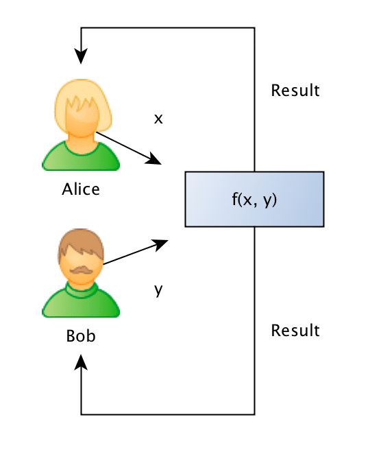
The Yao’s Millionaires Problem is where two millionaires, Alice and Bob, who are interested in knowing which of them is richer but without revealing to each other their actual wealth. In other words, what they want can be generalized as that: Alice and Bob want jointly compute a function securely, without knowing anything other than the result of the computation on the input data (that remains private to them).
To make the problem concrete, Alice has an amount A such as $10, and Bob has an amount B such as $ 50, and what they want to know is which one is larger, without Bob revealing the amount B to Alice or Alice revealing the amount A to Bob. It is also important to note that we also don’t want to trust on a third-party, otherwise the problem would just be a simple protocol of information exchange with the trusted party.
Formally what we want is to jointly evaluate the following function:
Such as the private values A and B are held private to the sole owner of it and where the result r will be known to just one or both of the parties.
It seems very counterintuitive that a problem like that could ever be solved, but for the surprise of many people, it is possible to solve it on some security requirements. Thanks to the recent developments in techniques such as FHE (Fully Homomorphic Encryption), Oblivious Transfer, Garbled Circuits, problems like that started to get practical for real-life usage and they are being nowadays being used by many companies in applications such as information exchange, secure location, advertisement, satellite orbit collision avoidance, etc.
I’m not going to enter into details of these techniques, but if you’re interested in the intuition behind the OT (Oblivious Transfer), you should definitely read the amazing explanation done by Craig Gidney here. There are also, of course, many different protocols for doing 2PC or MPC, where each one of them assumes some security requirements (semi-honest, malicious, etc), I’m not going to enter into the details to keep the post focused on the goal, but you should be aware of that.
The problem: sentence similarity
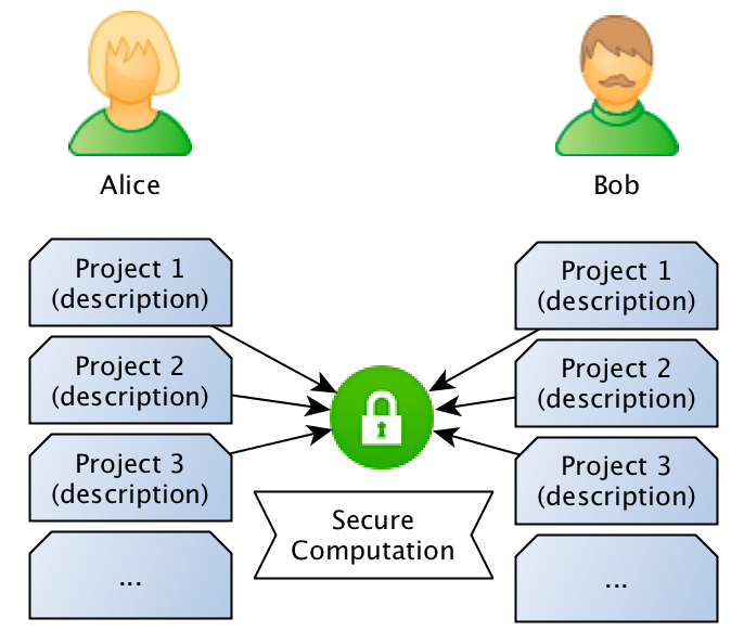
What we want to achieve is to use privacy-preserving computation to calculate the similarity between sentences without disclosing the content of the sentences. Just to give a concrete example: Bob owns a company and has the description of many different projects in sentences such as: “This project is about building a deep learning sentiment analysis framework that will be used for tweets“, and Alice who owns another competitor company, has also different projects described in similar sentences. What they want to do is to jointly compute the similarity between projects in order to find if they should be doing partnership on a project or not, however, and this is the important point: Bob doesn’t want Alice to know the project descriptions and neither Alice wants Bob to be aware of their projects, they want to know the closest match between the different projects they run, but without disclosing the project ideas (project descriptions).
Sentence Similarity Comparison
Now, how can we exchange information about the Bob and Alice’s project sentences without disclosing information about the project descriptions ?
One naive way to do that would be to just compute the hashes of the sentences and then compare only the hashes to check if they match. However, this would assume that the descriptions are exactly the same, and besides that, if the entropy of the sentences is small (like small sentences), someone with reasonable computation power can try to recover the sentence.
Another approach for this problem (this is the approach that we’ll be using), is to compare the sentences in the sentence embeddings space. We just need to create sentence embeddings using a Machine Learning model (we’ll use InferSent later) and then compare the embeddings of the sentences. However, this approach also raises another concern: what if Bob or Alice trains a Seq2Seq model that would go from the embeddings of the other party back to an approximate description of the project ?
It isn’t unreasonable to think that one can recover an approximate description of the sentence given their embeddings. That’s why we’ll use the two-party secure computation for computing the embeddings similarity, in a way that Bob and Alice will compute the similarity of the embeddings without revealing their embeddings, keeping their project ideas safe.
The entire flow is described in the image below, where Bob and Alice shares the same Machine Learning model, after that they use this model to go from sentences to embeddings, followed by a secure computation of the similarity in the embedding space.
Diagram overview of the entire process.
Generating sentence embeddings with InferSent
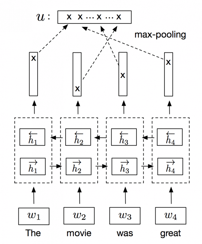
Bi-LSTM max-pooling network. Source: Supervised Learning of Universal Sentence Representations from Natural Language Inference Data. Alexis Conneau et al.
InferSent is an NLP technique for universal sentence representation developed by Facebook that uses supervised training to produce high transferable representations.
They used a Bi-directional LSTM with attention that consistently surpassed many unsupervised training methods such as the SkipThought vectors. They also provide a Pytorch implementation that we’ll use to generate sentence embeddings.
Note: even if you don’t have GPU, you can have reasonable performance doing embeddings for a few sentences.
The first step to generate the sentence embeddings is to download and load a pre-trained InferSent model:
import numpy as np
import torch

# Trained model from: https://github.com/facebookresearch/InferSent
GLOVE_EMBS = '../dataset/GloVe/glove.840B.300d.txt'
INFERSENT_MODEL = 'infersent.allnli.pickle'

# Load trained InferSent model
model = torch.load(INFERSENT_MODEL,
                   map_location=lambda storage, loc: storage)

model.set_glove_path(GLOVE_EMBS)
model.build_vocab_k_words(K=100000)
As you can see, if we have two unit vectors (vectors with norm 1), the two terms in the equation denominator will be 1 and we will be able to remove the entire denominator of the equation, leaving only:
So, if we normalize our vectors to have a unit norm (that’s why the vectors are wearing hats in the equation above), we can make the computation of the cosine similarity become just a simple dot product. That will help us a lot in computing the similarity distance later when we’ll use a framework to do the secure computation of this dot product.
So, the next step is to define a function that will take some sentence text and forward it to the model to generate the embeddings and then normalize them to unit vectors:
# This function will forward the text into the model and
# get the embeddings. After that, it will normalize it
# to a unit vector.

def encode(model, text):
    embedding = model.encode([text])[0]
    embedding /= np.linalg.norm(embedding)
    return embedding
As you can see, this function is pretty simple, it feeds the text into the model, and then it will divide the embedding vector by the embedding norm.
Now, for practical reasons, I’ll be using integer computation later for computing the similarity, however, the embeddings generated by InferSent are of course real values. For that reason, you’ll see in the code below that we create another function to scale the float values and remove the radix point andconverting them to integers. There is also another important issue, the framework that we’ll be using later for secure computation doesn’t allow signed integers, so we also need to clip the embeddings values between 0.0 and 1.0. This will of course cause some approximation errors, however, we can still get very good approximations after clipping and scaling with limited precision (I’m using 14 bits for scaling to avoid overflow issues later during dot product computations):
# This function will scale the embedding in order to
# remove the radix point.

def scale(embedding):
    SCALE = 1 << 14
    scale_embedding = np.clip(embedding, 0.0, 1.0) * SCALE
    return scale_embedding.astype(np.int32)
You can use floating-point in your secure computations and there are a lot of frameworks that support them, however, it is more tricky to do that, and for that reason, I used integer arithmetic to simplify the tutorial. The function above is just a hack to make it simple. It’s easy to see that we can recover this embedding later without too much loss of precision.
Now we just need to create some sentence samples that we’ll be using:
# The list of Alice sentences
alice_sentences = [
    'my cat loves to walk over my keyboard',
    'I like to pet my cat',
]

# The list of Bob sentences
bob_sentences = [
    'the cat is always walking over my keyboard',
]
And convert them to embeddings:
# Alice sentences
alice_sentence1 = encode(model, alice_sentences[0])
alice_sentence2 = encode(model, alice_sentences[1])

# Bob sentences
bob_sentence1 = encode(model, bob_sentences[0])
Since we have now the sentences and every sentence is also normalized, we can compute cosine similarity just by doing a dot product between the vectors:
As we can see, the first sentence of Bob is most similar (~0.87) with Alice first sentence than to the Alice second sentence (~0.62).
Since we have now the embeddings, we just need to convert them to scaled integers:
# Scale the Alice sentence embeddings
alice_sentence1_scaled = scale(alice_sentence1)
alice_sentence2_scaled = scale(alice_sentence2)

# Scale the Bob sentence embeddings
bob_sentence1_scaled = scale(bob_sentence1)

# This is the unit vector embedding for the sentence
>>> alice_sentence1
array([ 0.01698913, -0.0014404 ,  0.0010993 , ...,  0.00252409,
        0.00828147,  0.00466533], dtype=float32)

# This is the scaled vector as integers
>>> alice_sentence1_scaled
array([278,   0,  18, ...,  41, 135,  76], dtype=int32)
Now with these embeddings as scaled integers, we can proceed to the second part, where we’ll be doing the secure computation between two parties.
Two-party secure computation
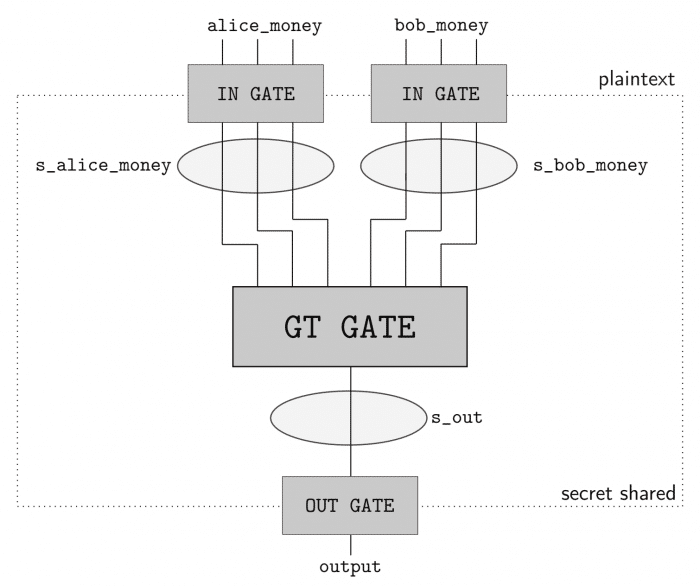
In order to perform secure computation between the two parties (Alice and Bob), we’ll use the ABY framework. ABY implements many difference secure computation schemes and allows you to describe your computation as a circuit like pictured in the image below, where the Yao’s Millionaire’s problem is described:
Yao’s Millionaires problem. Taken from ABY documentation (https://github.com/encryptogroup/ABY).
As you can see, we have two inputs entering in one GT GATE (greater than gate) and then a output. This circuit has a bit length of 3 for each input and will compute if the Alice input is greater than (GT GATE) the Bob input. The computing parties then secret share their private data and then can use arithmetic sharing, boolean sharing, or Yao sharing to securely evaluate these gates.
ABY is really easy to use because you can just describe your inputs, shares, gates and it will do the rest for you such as creating the socket communication channel, exchanging data when needed, etc. However, the implementation is entirely written in C++ and I’m not aware of any Python bindings for it (a great contribution opportunity).
Fortunately, there is an implemented example for ABY that can do dot product calculation for us, the example is here. I won’t replicate the example here, but the only part that we have to change is to read the embedding vectors that we created before instead of generating random vectors and increasing the bit length to 32-bits.
After that, we just need to execute the application on two different machines (or by emulating locally like below):
# This will execute the server part, the -r 0 specifies the role (server)
# and the -n 4096 defines the dimension of the vector (InferSent generates
# 4096-dimensional embeddings).
~# ./innerproduct -r 0 -n 4096

# And the same on another process (or another machine, however for another
# machine execution you'll have to obviously specify the IP).
~# ./innerproduct -r 1 -n 4096
And we get the following results:
Inner Product of alice_sentence1 and bob_sentence1  = 226691917
Inner Product of alice_sentence2 and bob_sentence1  = 171746521
Even in the integer representation, you can see that the inner product of the Alice’s first sentence and the Bob sentence is higher, meaning that the similarity is also higher. But let’s now convert this value back to float:
>>> SCALE = 1 << 14

# This is the dot product we should get
>>> np.dot(alice_sentence1, bob_sentence1)
0.8798542

# This is the inner product we got on secure computation
>>> 226691917 / SCALE**2.0
0.8444931

# This is the dot product we should get
>>> np.dot(alice_sentence2, bob_sentence1)
0.6297632

# This is the inner product we got on secure computation
>>> 171746521 / SCALE**2.0
0.6398056
As you can see, we got very good approximations, even in presence of low-precision math and unsigned integer requirements. Of course that in real-life you won’t have the two values and vectors, because they’re supposed to be hidden, but the changes to accommodate that are trivial, you just need to adjust ABY code to load only the vector of the party that it is executing it and using the correct IP addresses/port of the both parties.
The GIMPS (Great Internet Mersenne Prime Search) has confirmed yesterday the new largest known prime number: 277,232,917-1. This new largest known prime has 23,249,425 digits and is, of course, a Mersenne prime, prime numbers expressed in the form of 2n – 1, where the primality can be efficiently calculated using Lucas-Lehmer primality test.
One of the most asked questions about these largest primes is how the number of digits is calculated, given the size of these numbers (23,249,425 digits for the new largest known prime). And indeed there is a trick that avoids you to evaluate the number to calculate the number of digits, using Python you can just do:
>>> import numpy as np
>>> a = 2
>>> b = 77232917
>>> num_digits = int(1 + b * np.log10(a))
>>> print(num_digits)
23249425
The reason why this works is that the log base 10 of a number is how many times this number should be divided by 10 to get to 1, so you get the number of digits after 1 and just need to add 1 back.
Another interesting fact is that we can also get the last digit of this very large number again without evaluating the entire number by using congruence. Since we’re interested in the number mod 10 and we know that the Mersenne prime has the form of 277,232,917-1, we can check that the powers 2n have an easy cycling pattern:
(… repeat)
Which means that powers of 2 mod 10 repeats at every 4 numbers, thus we just need to compute 77,232,917 mod 4, which is 1. Given that the part 277,232,917 ends in 2 and when you subtract 1 you end up with 1 as the last digit, as you can confirm by looking at the entire number (~10Mb zipfile).
Since Benford’s law got some attention in the past years, I decided to make a list of the previous posts I made on the subject in the context of elections, fraud, corruption, universality and prime numbers:
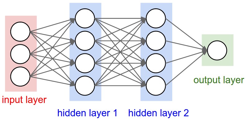
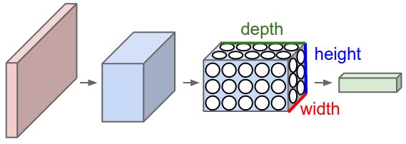
Convolutional neural networks (or ConvNets) are biologically-inspired variants of MLPs, they have different kinds of layers and each different layer works different than the usual MLP layers. If you are interested in learning more about ConvNets, a good course is the CS231n – Convolutional Neural Newtorks for Visual Recognition. The architecture of the CNNs are shown in the images below:
As you can see, the ConvNets works with 3D volumes and transformations of these 3D volumes. I won’t repeat in this post the entire CS231n tutorial, so if you’re really interested, please take time to read before continuing.
Lasagne and nolearn
One of the Python packages for deep learning that I really like to work with is Lasagne and nolearn. Lasagne is based on Theano so the GPU speedups will really make a great difference, and their declarative approach for the neural networks creation are really helpful. The nolearn libary is a collection of utilities around neural networks packages (including Lasagne) that can help us a lot during the creation of the neural network architecture, inspection of the layers, etc.
What I’m going to show in this post, is how to build a simple ConvNet architecture with some convolutional and pooling layers. I’m also going to show how you can use a ConvNet to train a feature extractor and then use it to extract features before feeding them into different models like SVM, Logistic Regression, etc. Many people use pre-trained ConvNet models and then remove the last output layer to extract the features from ConvNets that were trained on ImageNet datasets. This is usually called transfer learning because you can use layers from other ConvNets as feature extractors for different problems, since the first layer filters of the ConvNets works as edge detectors, they can be used as general feature detectors for other problems.
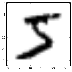
Loading the MNIST dataset
The MNIST dataset is one of the most traditional datasets for digits classification. We will use a pickled version of it for Python, but first, lets import the packages that we will need to use:
import matplotlib
import matplotlib.pyplot as plt
import matplotlib.cm as cm
from urllib import urlretrieve
import cPickle as pickle
import os
import gzip
import numpy as np
import theano
import lasagne
from lasagne import layers
from lasagne.updates import nesterov_momentum
from nolearn.lasagne import NeuralNet
from nolearn.lasagne import visualize
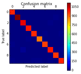
from sklearn.metrics import classification_report
from sklearn.metrics import confusion_matrix
As you can see, we are importing matplotlib for plotting some images, some native Python modules to download the MNIST dataset, numpy, theano, lasagne, nolearn and some scikit-learn functions for model evaluation.
After that, we define our MNIST loading function (this is pretty the same function used in the Lasagne tutorial):
As you can see, we are downloading the MNIST pickled dataset and then unpacking it into the three different datasets: train, validation and test. After that we reshape the image contents to prepare them to input into the Lasagne input layer later and we also convert the numpy array types to uint8 due to the GPU/theano datatype restrictions.
After that, we’re ready to load the MNIST dataset and inspect it:
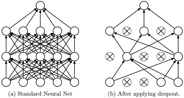
As you can see, in the parameter layers we’re defining a dictionary of tuples with the layer names/types and then we define the parameters for these layers. Our architecture here is using two convolutional layers with poolings and then a fully connected layer (dense layer) and the output layer. There are also dropouts between some layers, the dropout layer is a regularizer that randomly sets input values to zero to avoid overfitting (see the image below).
Dropout layer effect (from CS231n website).
After calling the train method, the nolearn package will show status of the learning process, in my machine with my humble GPU I got the results below:
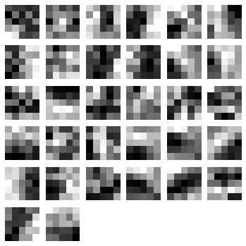
The code above will plot the following filters below:
The first layer 5x5x32 filters.
As you can see, the nolearn plot_conv_weights plots all the filters present in the layer we specified.
Theano layer functions and Feature Extraction
Now it is time to create theano-compiled functions that will feed-forward the input data into the architecture up to the layer you’re interested. I’m going to get the functions for the output layer and also for the dense layer before the output layer:
As you can see, we have now two theano functions called f_output and f_dense (for the output and dense layers). Please note that in order to get the layers here we are using a extra parameter called “deterministic“, this is to avoid the dropout layers affecting our feed-forward pass.
We can now convert an example instance to the input format and then feed it into the theano function for the output layer:
instance = X_test[0][None, :, :]
%timeit -n 500 f_output(instance)

500 loops, best of 3: 858 µs per loop
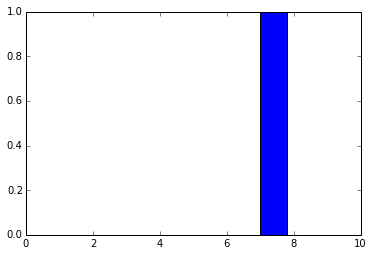
As you can see, the f_output function takes an average of 858 µs. We can also plot the output layer activations for the instance:
pred = f_output(instance)
N = pred.shape[1]
plt.bar(range(N), pred.ravel())
The code above will create the following plot:
Output layer activations.
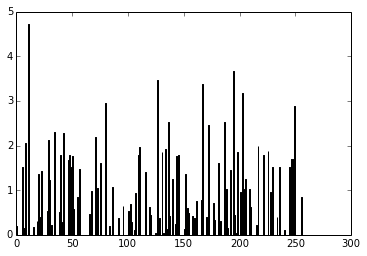
As you can see, the digit was recognized as the digit 7. The fact that you can create theano functions for any layer of the network is very useful because you can create a function (like we did before) to get the activations for the dense layer (the one before the output layer) and you can use these activations as features and use your neural network not as classifier but as a feature extractor. Let’s plot now the 256 unit activations for the dense layer:
pred = f_dense(instance)
N = pred.shape[1]
plt.bar(range(N), pred.ravel())
The code above will create the following plot below:
Dense layer activations.
You can now use the output of the these 256 activations as features on a linear classifier like Logistic Regression or SVM.
Update – 05 Dec 2017: Google just announced that it will be commited to the development of a new released version of the S2 library, amazing news, repository can be found here.
Google’s S2 library is a real treasure, not only due to its capabilities for spatial indexing but also because it is a library that was released more than 4 years ago and it didn’t get the attention it deserved. The S2 library is used by Google itself on Google Maps, MongoDB engine and also by Foursquare, but you’re not going to find any documentation or articles about the library anywhere except for a paper by Foursquare, a Google presentation and the source code comments. You’ll also struggle to find bindings for the library, the official repository has missing Swig files for the Python library and thanks to some forks we can have a partial binding for the Python language (I’m going to it use for this post). I heard that Google is actively working on the library right now and we are probably soon going to get more details about it when they release this work, but I decided to share some examples about the library and the reasons why I think that this library is so cool.
The way to the cells
You’ll see this “cell” concept all around the S2 code. The cells are an hierarchical decomposition of the sphere (the Earth on our case, but you’re not limited to it) into compact representations of regions or points. Regions can also be approximated using these same cells, that have some nice features:
They are compact (represented by 64-bit integers)
They have resolution for geographical features
They are hierarchical (thay have levels, and similar levels have similar areas)
The containment query for arbitrary regions are really fast
The S2 library starts by projecting the points/regions of the sphere into a cube, and each face of the cube has a quad-tree where the sphere point is projected into. After that, some transformation occurs (for more details on why, see the Google presentation) and the space is discretized, after that the cells are enumerated on a Hilbert Curve, and this is why this library is so nice, the Hilbert curve is a space-filling curve that converts multiple dimensions into one dimension that has an special spatial feature: it preserves the locality.
Hilbert Curve
Hilbert Curve
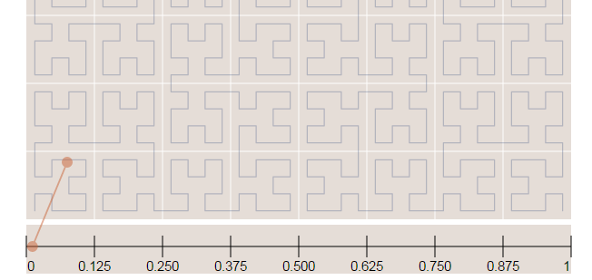
The Hilbert curve is space-filling curve, which means that its range covers the entire n-dimensional space. To understand how this works, you can imagine a long string that is arranged on the space in a special way such that the string passes through each square of the space, thus filling the entire space. To convert a 2D point along to the Hilbert curve, you just need select the point on the string where the point is located. An easy way to understand it is to use this iterative example where you can click on any point of the curve and it will show where in the string the point is located and vice-versa.
In the image below, the point in the very beggining of the Hilbert curve (the string) is located also in the very beginning along curve (the curve is represented by a long string in the bottom of the image):
Hilbert Curve
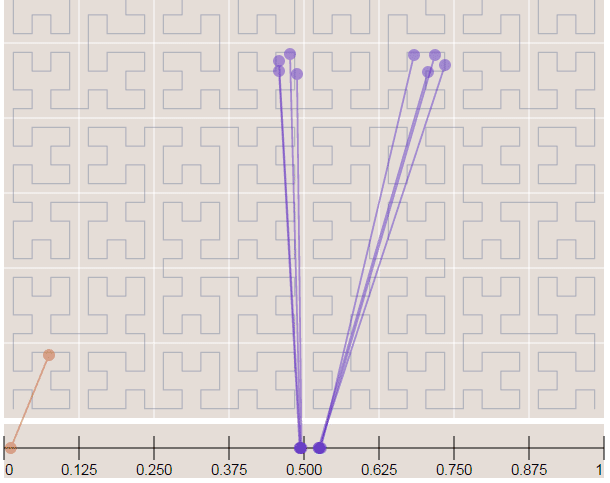
Now in the image below where we have more points, it is easy to see how the Hilbert curve is preserving the spatial locality. You can note that points closer to each other in the curve (in the 1D representation, the line in the bottom) are also closer in the 2D dimensional space (in the x,y plane). However, note that the opposite isn’t quite true because you can have 2D points that are close to each other in the x,y plane that aren’t close in the Hilbert curve.
Hilbert Curve
Since S2 uses the Hilbert Curve to enumerate the cells, this means that cell values close in value are also spatially close to each other. When this idea is combined with the hierarchical decomposition, you have a very fast framework for indexing and for query operations. Before we start with the pratical examples, let’s see how the cells are represented in 64-bit integers.
If you are interested in Hilbert Curves, I really recommend this article, it is very intuitive and show some properties of the curve.
The cell representation
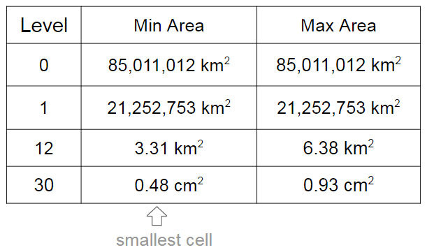
As I already mentioned, the cells have different levels and different regions that they can cover. In the S2 library you’ll find 30 levels of hierachical decomposition. The cell level and the area range that they can cover is shown in the Google presentation in the slide that I’m reproducing below:
Cell areas
As you can see, a very cool result of the S2 geometry is that every cm² of the earth can be represented using a 64-bit integer.
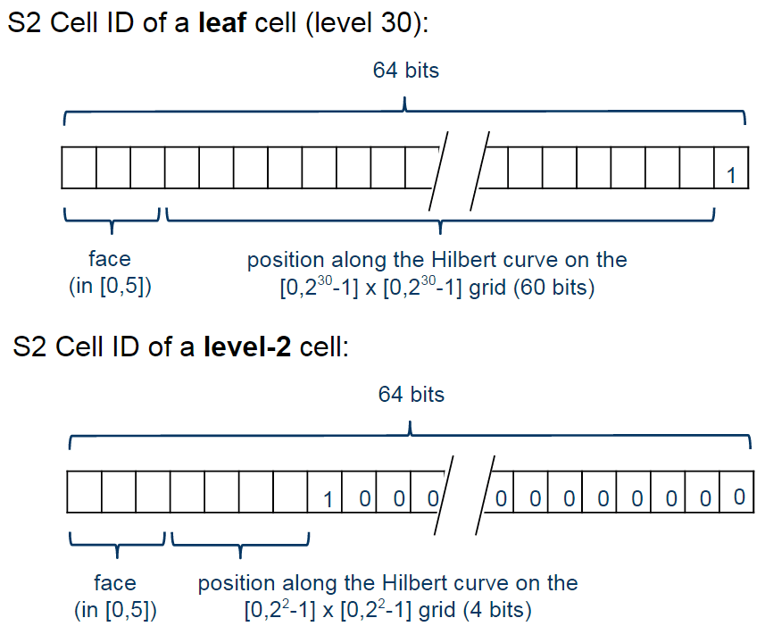
The cells are represented using the following schema:
Cell Representation Schema (images from the original Google presentation)
The first one is representing a leaf cell, a cell with the minimum area usually used to represent points. As you can see, the 3 initial bits are reserved to store the face of the cube where the point of the sphere was projected, then it is followed by the position of the cell in the Hilbert curve always followed by a “1” bit that is a marker that will identify the level of the cell.
So, to check the level of the cell, all that is required is to check where the last “1” bit is located in the cell representation. The checking of containment, to verify if a cell is contained in another cell, all you just have to do is to do a prefix comparison. These operations are really fast and they are possible only due to the Hilbert Curve enumeration and the hierarchical decomposition method used.
Covering regions
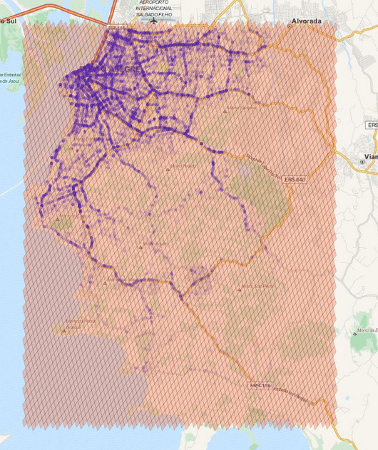
So, if you want to generate cells to cover a region, you can use a method of the library where you specify the maximum number of the cells, the maximum cell level and the minimum cell level to be used and an algorithm will then approximate this region using the specified parameters. In the example below, I’m using the S2 library to extract some Machine Learning binary features using level 15 cells:
Cells at level 15 – binary features for Machine Learning
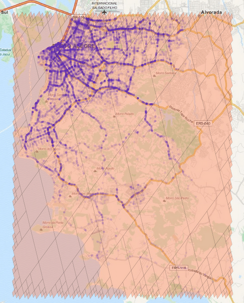
The cells regions are here represented in the image above using transparent polygons over the entire region of interest of my city. Since I used the level 15 both for minimum and maximum level, the cells are all covering similar region areas. If I change the minimum level to 8 (thus allowing the possibility of using larger cells), the algorithm will approximate the region in a way that it will provide the smaller number of cells and also trying to keep the approximation precise like in the example below:
Covering using range from 8 to 15 (levels)
As you can see, we have now a covering using larger cells in the center and to cope with the borders we have an approximation using smaller cells (also note the quad-trees).
Examples
* In this tutorial I used the Python 2.7 bindings from the following repository. The instructions to compile and install it are present in the readme of the repository so I won’t repeat it here.
The first step to convert Latitude/Longitude points to the cell representation are shown below:
As you can see, we first create an object of the class S2LatLng to represent the lat/lng point and then we feed it into the S2CellId class to build the cell representation. After that, we can get the level and id of the class. There is also a method called ToToken that converts the integer representation to a compact alphanumerical representation that you can parse it later using FromToken method.
You can also get the parent cell of that cell (one level above it) and use containment methods to check if a cell is contained by another cell:
As you can see, the level of the parent is one above the children cell (in our case, a leaf cell). The ids are also very similar except for the level of the cell and the containment checking is really fast (it is only checking the range of the children cells of the parent cell).
These cells can be stored on a database and they will perform quite well on a BTree index. In order to create a collection of cells that will cover a region, you can use the S2RegionCoverer class like in the example below:
First of all, we defined a S2LatLngRect which is a rectangle delimiting the region that we want to cover. There are also other classes that you can use (to build polygons for instance), the S2RegionCoverer works with classes that uses the S2Region class as base class. After defining the rectangle, we instantiate the S2RegionCoverer and then set the aforementioned min/max levels and the max number of the cells that we want the approximation to generate.
If you wish to plot the covering, you can use Cartopy, Shapely and matplotlib, like in the example below:
import matplotlib.pyplot as plt

from s2 import *

from shapely.geometry import Polygon

import cartopy.crs as ccrs
import cartopy.io.img_tiles as cimgt

proj = cimgt.MapQuestOSM()
plt.figure(figsize=(20,20), dpi=200)
ax = plt.axes(projection=proj.crs)

ax.add_image(proj, 12)
ax.set_extent([-51.411886, -50.922470,
               -30.301314, -29.94364])

region_rect = S2LatLngRect(
    S2LatLng.FromDegrees(-51.264871, -30.241701),
    S2LatLng.FromDegrees(-51.04618, -30.000003))

coverer = S2RegionCoverer()
coverer.set_min_level(8)
coverer.set_max_level(15)
coverer.set_max_cells(500)
covering = coverer.GetCovering(region_rect)

geoms = []
for cellid in covering:
    new_cell = S2Cell(cellid)
    vertices = []
    for i in xrange(0, 4):
        vertex = new_cell.GetVertex(i)
        latlng = S2LatLng(vertex)
        vertices.append((latlng.lat().degrees(),
                         latlng.lng().degrees()))

    geo = Polygon(vertices)
    geoms.append(geo)

print "Total Geometries: {}".format(len(geoms))

ax.add_geometries(geoms, ccrs.PlateCarree(), facecolor='coral',
                  edgecolor='black', alpha=0.4)
plt.show()
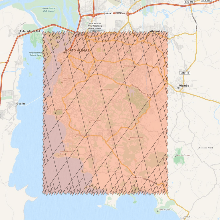
And the result will be the one below:
The covering cells.
There are a lot of stuff in the S2 API, and I really recommend you to explore and read the source-code, it is really helpful. The S2 cells can be used for indexing and in key-value databases, it can be used on B Trees with really good efficiency and also even for Machine Learning purposes (which is my case), anyway, it is a very useful tool that you should keep in your toolbox. I hope you enjoyed this little tutorial !
This website uses cookies to improve your experience. We'll assume you're ok with this, but you can opt-out if you wish. Cookie settingsACCEPT
Privacy & Cookies Policy
Privacy Overview
This website uses cookies to improve your experience while you navigate through the website. Out of these cookies, the cookies that are categorized as necessary are stored on your browser as they are essential for the working of basic functionalities of the website. We also use third-party cookies that help us analyze and understand how you use this website. These cookies will be stored in your browser only with your consent. You also have the option to opt-out of these cookies. But opting out of some of these cookies may have an effect on your browsing experience.
Necessary cookies are absolutely essential for the website to function properly. This category only includes cookies that ensures basic functionalities and security features of the website. These cookies do not store any personal information.
Any cookies that may not be particularly necessary for the website to function and is used specifically to collect user personal data via analytics, ads, other embedded contents are termed as non-necessary cookies. It is mandatory to procure user consent prior to running these cookies on your website.

")
 What they want to do is to jointly compute the similarity between projects in order to find if they should be doing partnership on a project or not, however, and this is the important point: Bob doesn’t want Alice to know the project descriptions and neither Alice wants Bob to be aware of their projects, they want to know the closest match between the different projects they run, but without disclosing the project ideas (project descriptions).
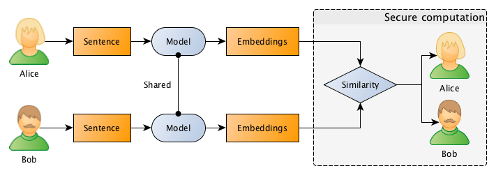
 = \frac {\pmb x \cdot \pmb y}{||\pmb x|| \cdot ||\pmb y||}")
 =\hat{x} \cdot\hat{y}")


 the part 277,232,917 ends in 2 and when you subtract 1 you end up with 1 as the last digit, as you can confirm by looking at the