Programming

Machine Learning, Programming, Python

Machine Learning :: Cosine Similarity for Vector Space Models (Part III)

* It has been a long time since I wrote the TF-IDF tutorial (Part I and Part II) and as I promissed, here is the continuation of the tutorial. Unfortunately I had no time to fix the previous tutorials for the newer versions of the scikit-learn (sklearn) package nor to answer all the questions, but I hope to do that in a close future.

So, on the previous tutorials we learned how a document can be modeled in the Vector Space, how the TF-IDF transformation works and how the TF-IDF is calculated, now what we are going to learn is how to use a well-known similarity measure (Cosine Similarity) to calculate the similarity between different documents.

The Dot Product

Let’s begin with the definition of the dot product for two vectors: \vec{a} = (a_1, a_2, a_3, \ldots) and \vec{b} = (b_1, b_2, b_3, \ldots), where a_n and b_n are the components of the vector (features of the document, or TF-IDF values for each word of the document in our example) and the \mathit{n} is the dimension of the vectors:

  \vec{a} \cdot \vec{b} = \sum_{i=1}^n a_ib_i = a_1b_1 + a_2b_2 + \cdots + a_nb_n

As you can see, the definition of the dot product is a simple multiplication of each component from the both vectors added together. See an example of a dot product for two vectors with 2 dimensions each (2D):

  \vec{a} = (0, 3) \\   \vec{b} = (4, 0) \\   \vec{a} \cdot \vec{b} = 0*4 + 3*0 = 0

The first thing you probably noticed is that the result of a dot product between two vectors isn’t another vector but a single value, a scalar.

This is all very simple and easy to understand, but what is a dot product ? What is the intuitive idea behind it ? What does it mean to have a dot product of zero ? To understand it, we need to understand what is the geometric definition of the dot product:

  \vec{a} \cdot \vec{b} = \|\vec{a}\|\|\vec{b}\|\cos{\theta}

Rearranging the equation to understand it better using the commutative property, we have:

  \vec{a} \cdot \vec{b} = \|\vec{b}\|\|\vec{a}\|\cos{\theta}

So, what is the term \displaystyle \|\vec{a}\|\cos{\theta} ? This term is the projection of the vector \vec{a} into the vector \vec{b} as shown on the image below:

The projection of the vector A into the vector B. By Wikipedia.

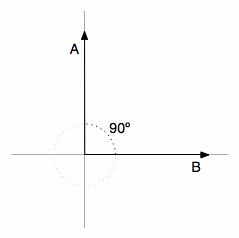
Now, what happens when the vector \vec{a} is orthogonal (with an angle of 90 degrees) to the vector \vec{b} like on the image below ?

Two orthogonal vectors (with 90 degrees angle).

There will be no adjacent side on the triangle, it will be equivalent to zero, the term \displaystyle \|\vec{a}\|\cos{\theta} will be zero and the resulting multiplication with the magnitude of the vector \vec{b} will also be zero. Now you know that, when the dot product between two different vectors is zero, they are orthogonal to each other (they have an angle of 90 degrees), this is a very neat way to check the orthogonality of different vectors. It is also important to note that we are using 2D examples, but the most amazing fact about it is that we can also calculate angles and similarity between vectors in higher dimensional spaces, and that is why math let us see far than the obvious even when we can’t visualize or imagine what is the angle between two vectors with twelve dimensions for instance.

The Cosine Similarity

The cosine similarity between two vectors (or two documents on the Vector Space) is a measure that calculates the cosine of the angle between them. This metric is a measurement of orientation and not magnitude, it can be seen as a comparison between documents on a normalized space because we’re not taking into the consideration only the magnitude of each word count (tf-idf) of each document, but the angle between the documents. What we have to do to build the cosine similarity equation is to solve the equation of the dot product for the \cos{\theta}:

  \displaystyle  \vec{a} \cdot \vec{b} = \|\vec{a}\|\|\vec{b}\|\cos{\theta} \\ \\  \cos{\theta} = \frac{\vec{a} \cdot \vec{b}}{\|\vec{a}\|\|\vec{b}\|}

And that is it, this is the cosine similarity formula. Cosine Similarity will generate a metric that says how related are two documents by looking at the angle instead of magnitude, like in the examples below:

The Cosine Similarity values for different documents, 1 (same direction), 0 (90 deg.), -1 (opposite directions).

Note that even if we had a vector pointing to a point far from another vector, they still could have an small angle and that is the central point on the use of Cosine Similarity, the measurement tends to ignore the higher term count on documents. Suppose we have a document with the word “sky” appearing 200 times and another document with the word “sky” appearing 50, the Euclidean distance between them will be higher but the angle will still be small because they are pointing to the same direction, which is what matters when we are comparing documents.

Now that we have a Vector Space Model of documents (like on the image below) modeled as vectors (with TF-IDF counts) and also have a formula to calculate the similarity between different documents in this space, let’s see now how we do it in practice using scikit-learn (sklearn).
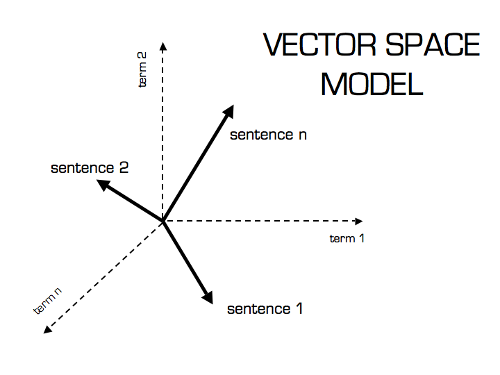
Vector Space Model

Practice Using Scikit-learn (sklearn)

* In this tutorial I’m using the Python 2.7.5 and Scikit-learn 0.14.1.

The first thing we need to do is to define our set of example documents:

documents = (
"The sky is blue",
"The sun is bright",
"The sun in the sky is bright",
"We can see the shining sun, the bright sun"
)

And then we instantiate the Sklearn TF-IDF Vectorizer and transform our documents into the TF-IDF matrix:

from sklearn.feature_extraction.text import TfidfVectorizer
tfidf_vectorizer = TfidfVectorizer()
tfidf_matrix = tfidf_vectorizer.fit_transform(documents)
print tfidf_matrix.shape
(4, 11)

Now we have the TF-IDF matrix (tfidf_matrix) for each document (the number of rows of the matrix) with 11 tf-idf terms (the number of columns from the matrix), we can calculate the Cosine Similarity between the first document (“The sky is blue”) with each of the other documents of the set:

from sklearn.metrics.pairwise import cosine_similarity
cosine_similarity(tfidf_matrix[0:1], tfidf_matrix)
array([[ 1.        ,  0.36651513,  0.52305744,  0.13448867]])

The tfidf_matrix[0:1] is the Scipy operation to get the first row of the sparse matrix and the resulting array is the Cosine Similarity between the first document with all documents in the set. Note that the first value of the array is 1.0 because it is the Cosine Similarity between the first document with itself. Also note that due to the presence of similar words on the third document (“The sun in the sky is bright”), it achieved a better score.

If you want, you can also solve the Cosine Similarity for the angle between vectors:

  \cos{\theta} = \frac{\vec{a} \cdot \vec{b}}{\|\vec{a}\|\|\vec{b}\|}

We only need to isolate the angle (\theta) and move the \cos to the right hand of the equation:

  \theta = \arccos{\frac{\vec{a} \cdot \vec{b}}{\|\vec{a}\|\|\vec{b}\|}}

The \arccos is the same as the inverse of the cosine (\cos^-1).

 Lets for instance, check the angle between the first and third documents:
import math
# This was already calculated on the previous step, so we just use the value
cos_sim = 0.52305744
angle_in_radians = math.acos(cos_sim)
print math.degrees(angle_in_radians)
58.462437107432784

And that angle of ~58.5 is the angle between the first and the third document of our document set.

That is it, I hope you liked this third tutorial !
Cite this article as: Christian S. Perone, "Machine Learning :: Cosine Similarity for Vector Space Models (Part III)," in Terra Incognita, 12/09/2013, https://blog.christianperone.com/2013/09/machine-learning-cosine-similarity-for-vector-space-models-part-iii/.

Related Material

A video about Dot Product on The Khan Academy

Wikipedia: Dot Product

Wikipedia: Cosine Similarity

Scikit-learn (sklearn) – The de facto Machine Learning package for Python
Programming, Python

Accessing HP Cloud OpenStack Nova using Python and Requests

So, my request to enter on the free and private beta season of the new HP Cloud Services was gently accepted by the HP Cloud team, and today I finally got some time to play with the OpenStack API at HP Cloud. I’ll start with the first impressions I had with the service:

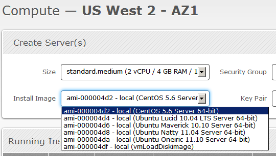
The user interface of the management is very user-friendly, the design is much like of the Twitter Bootstrap, see the screenshot below of the “Compute” page from the “Manage” section:

As you can see, they have a set of 4 Ubuntu images and a CentOS, I think that since they are still in the beta period, soon we’ll have more default images to use.

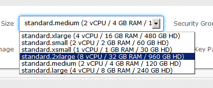
Here is a screenshot of the instance size set:

Since they are using OpenStack, I really think that they should have imported the vocabulary of the OpenStack into the user interface, and instead of calling it “Size”, it would be more sensible to use “Flavour“.

The user interface still doesn’t have many features, something that I would really like to have is a “Stop” or something like that for the instances, only the “Terminate” function is present on the Manage interface, but those are details that they should be still working on since they’re only in beta.

Another important info to cite is that the access to the instances are done through SSH using a generated RSA key that they provide to you.

Let’s dig into the OpenStack API now.

OpenStack API

To access the OpenStack API you’ll need the credentials for the authentication, HP Cloud services provide these keys on the Manage interface for each zone/service you have, see the screenshot below (with keys anonymized of course):

Now, OpenStack authentication could be done in different schemes, the scheme that I know that HP supports is the token authentication. I know that there is a lot of clients already supporting the OpenStack API (some have no documentation, some have weird API design, etc.), but the aim of this post is to show how easy would be to create a simple interface to access the OpenStack API using Python and Requests (HTTP for Humans !).

Let’s start defining our authentication scheme by sub-classing Requests AuthBase:

[enlighter lang=”python” ]
class OpenStackAuth(AuthBase):
def __init__(self, auth_user, auth_key):
self.auth_key = auth_key
self.auth_user = auth_user

def __call__(self, r):
r.headers[‘X-Auth-User’] = self.auth_user
r.headers[‘X-Auth-Key’] = self.auth_key
return r
[/enlighter]

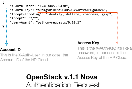
As you can see, we’re defining the X-Auth-User and the X-Auth-Key in the header of the request with the parameters. These parameters are respectively your Account ID and  Access Key we cited earlier. Now, all you have to do is to make the request itself using the authentication scheme, which is pretty easy using Requests:

[enlighter lang=”python”]
ENDPOINT_URL = ‘https://az-1.region-a.geo-1.compute.hpcloudsvc.com/v1.1/’
ACCESS_KEY = ‘Your Access Key’
ACCOUNT_ID = ‘Your Account ID’
response = requests.get(ENDPOINT_URL, auth=OpenStackAuth(ACCOUNT_ID, ACCESS_KEY))
[/enlighter]

And that is it, you’re done with the authentication mechanism using just a few lines of code, and this is how the request is going to be sent to the HP Cloud service server:

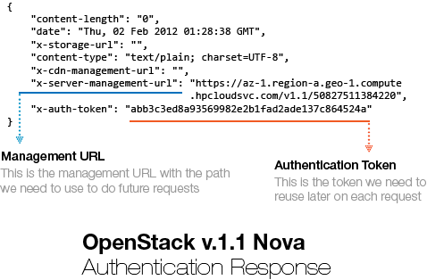
 This request is sent to the HP Cloud Endpoint URL (https://az-1.region-a.geo-1.compute.hpcloudsvc.com/v1.1/). Let’s see now how the server answered this authentication request:

You can show this authentication response using Requests by printing the header attribute of the request Response object. You can see that the server answered our request with two important header items: X-Server-Management-URL and the X-Auth-Token. The management URL is now our new endpoint, is the URL we should use to do further requests to the HP Cloud services and the X-Auth-Token is the authentication Token that the server generated based on our credentials, these tokens are usually valid for 24 hours, although I haven’t tested it.

What we need to do now is to sub-class the Requests AuthBase class again but this time defining only the authentication token that we need to use on each new request we’re going to make to the management URL:

[enlighter lang=”python”]
class OpenStackAuthToken(AuthBase):
def __init__(self, request):
self.auth_token = request.headers[‘x-auth-token’]

def __call__(self, r):
r.headers[‘X-Auth-Token’] = self.auth_token
return r
[/enlighter]

Note that the OpenStackAuthToken is receiving now a response request as parameter, copying the X-Auth-Token and setting it on the request.

Let’s consume a service from the OpenStack API v.1.1, I’m going to call the List Servers API function, parse the results using JSON and then show the results on the screen:

[enlighter lang=”python”]
# Get the management URL from the response header
mgmt_url = response.headers[‘x-server-management-url’]

# Create a new request to the management URL using the /servers path
# and the OpenStackAuthToken scheme we created
r_server = requests.get(mgmt_url + ‘/servers’, auth=OpenStackAuthToken(response))

# Parse the response and show it to the screen
json_parse = json.loads(r_server.text)
print json.dumps(json_parse, indent=4)
[/enlighter]

And this is what we get in response to this request:

[enlighter]
{
“servers”: [
{
“id”: 22378,
“uuid”: “e2964d51-fe98-48f3-9428-f3083aa0318e”,
“links”: [
{
“href”: “https://az-1.region-a.geo-1.compute.hpcloudsvc.com/v1.1/20817201684751/servers/22378”,
“rel”: “self”
},
{
“href”: “https://az-1.region-a.geo-1.compute.hpcloudsvc.com/20817201684751/servers/22378”,
“rel”: “bookmark”
}
],
“name”: “Server 22378”
},
{
“id”: 11921,
“uuid”: “312ff473-3d5d-433e-b7ee-e46e4efa0e5e”,
“links”: [
{
“href”: “https://az-1.region-a.geo-1.compute.hpcloudsvc.com/v1.1/20817201684751/servers/11921”,
“rel”: “self”
},
{
“href”: “https://az-1.region-a.geo-1.compute.hpcloudsvc.com/20817201684751/servers/11921”,
“rel”: “bookmark”
}
],
“name”: “Server 11921”
}
]
}
[/enlighter]

And that is it, now you know how to use Requests and Python to consume OpenStack API. If you wish to read more information about the API and how does it works, you can read the documentation here.

– Christian S. Perone