Programming

LLVM, Machine Learning, Programming, Python

JIT native code generation for TensorFlow computation graphs using Python and LLVM

Update: Hacker News discussion here.

The TensorFlow Computation Graph

tensorlogo

One of the most amazing components of the TensorFlow architecture is the computation graph that can be serialized using Protocol Buffers. This computation graph follows a well-defined format (click here for the proto files) and describes the computation that you specify (it can be a Deep Learning model like a CNN, a simple Logistic Regression or even any computation you want). For instance, here is an example of a very simple TensorFlow computation graph that we will use in this tutorial (using TensorFlow Python API):

import tensorflow as tf

with tf.Session() as sess:
    input_placeholder = tf.placeholder(tf.int32, 1, name="input")
    sub_op = tf.sub(input_placeholder, tf.constant(2, dtype=tf.int32))
    add_op = tf.add(sub_op, tf.constant(5, dtype=tf.int32))
    output = tf.add(add_op, tf.constant(100, dtype=tf.int32),
                    name="output")
    tf.train.write_graph(sess.graph_def, ".", "graph.pb", True)
Representation of the computation graph.

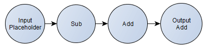
As you can see, this is a very simple computation graph. First, we define the placeholder that will hold the input tensor and after that we specify the computation that should happen using this input tensor as input data. Here we can also see that we’re defining two important nodes of this graph, one is called “input” (the aforementioned placeholder) and the other is called “output“, that will hold the result of the final computation. This graph is the same as the following formula for a scalar: output = (((input - 2)-5)+100), where I intentionally added redundant operations to see LLVM constant propagation later.

In the last line of the code, we’re persisting this computation graph (including the constant values) into a serialized protobuf file. The final True parameter is to output a textual representation instead of binary, so it will produce the following human-readable output protobuf file (I omitted a part of it for brevity):

node {
  name: "input"
  op: "Placeholder"
  attr {
    key: "dtype"
    value {
      type: DT_INT32
    }
  }
  attr {
    key: "shape"
    value {
      shape {
        dim {
          size: 1
        }
      }
    }
  }
}
node {
  name: "Const"
  op: "Const"
  attr {
    key: "dtype"
    value {
      type: DT_INT32
    }
  }
  attr {
    key: "value"
    value {
      tensor {
        dtype: DT_INT32
        tensor_shape {
        }
        int_val: 2
      }
    }
  }
}

--- >(omitted for brevity) < ---

node {
  name: "output"
  op: "Add"
  input: "Add"
  input: "Const_2"
  attr {
    key: "T"
    value {
      type: DT_INT32
    }
  }
}
versions {
  producer: 9
}

This is a very simple graph, and TensorFlow graphs are actually never that simple, because TensorFlow models can easily contain more than 300 nodes depending on the model you’re specifying, specially for Deep Learning models.

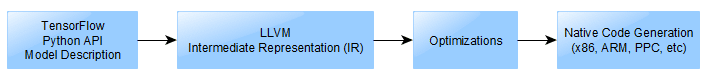
We’ll use the above graph to show how we can JIT native code for this simple graph using LLVM framework.

The LLVM Frontend, IR and Backend

LLVM-Logo-Derivative-1

The LLVM framework is a really nice, modular and complete ecosystem for building compilers and toolchains. A very nice description of the LLVM architecture that is important for us is shown in the picture below:

LLVM Compiler Architecture
LLVM Compiler Architecture (AOSA/LLVM, Chris Lattner)

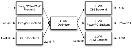
(The picture above is just a small part of the LLVM architecture, for a comprehensive description of it, please see the nice article from the AOSA book written by Chris Lattner)

Looking in the image above, we can see that LLVM provides a lot of core functionality, in the left side you see that many languages can write code for their respective language frontends, after that it doesn’t matter in which language you wrote your code, everything is transformed into a very powerful language called LLVM IR (LLVM Intermediate Representation) which is as you can imagine, a intermediate representation of the code just before the assembly code itself. In my opinion, the IR is the key component of what makes LLVM so amazing, because it doesn’t matter in which language you wrote your code (or even if it was a JIT’ed IR), everything ends in the same representation, and then here is where the magic happens, because the IR can take advantage of the LLVM optimizations (also known as transform and analysis passes).

After this IR generation, you can feed it into any LLVM backend to generate native code for any architecture supported by LLVM (such as x86, ARM, PPC, etc) and then you can finally execute your code with the native performance and also after LLVM optimization passes.

In order to JIT code using LLVM, all you need is to build the IR programmatically, create a execution engine to convert (during execution-time) the IR into native code, get a pointer for the function you have JIT’ed and then finally execute it. I’ll use here a Python binding for LLVM called llvmlite, which is very Pythonic and easy to use.

JIT’ing TensorFlow Graph using Python and LLVM

flow

Let’s now use the LLVM and Python to JIT the TensorFlow computational graph. This is by no means a comprehensive implementation, it is very simplistic approach, a oversimplification that assumes some things: a integer closure type, just some TensorFlow operations and also a single scalar support instead of high rank tensors.

So, let’s start building our JIT code; first of all, let’s import the required packages, initialize some LLVM sub-systems and also define the LLVM respective type for the TensorFlow integer type:

from ctypes import CFUNCTYPE, c_int

import tensorflow as tf
from google.protobuf import text_format
from tensorflow.core.framework import graph_pb2
from tensorflow.core.framework import types_pb2
from tensorflow.python.framework import ops

import llvmlite.ir as ll
import llvmlite.binding as llvm

llvm.initialize()
llvm.initialize_native_target()
llvm.initialize_native_asmprinter()

TYPE_TF_LLVM = {
    types_pb2.DT_INT32: ll.IntType(32),
}

After that, let’s define a class to open the TensorFlow exported graph and also declare a method to get a node of the graph by name:

class TFGraph(object):
    def __init__(self, filename="graph.pb", binary=False):
        self.graph_def = graph_pb2.GraphDef()
        with open("graph.pb", "rb") as f:
            if binary:
                self.graph_def.ParseFromString(f.read())
            else:
                text_format.Merge(f.read(), self.graph_def)

    def get_node(self, name):
        for node in self.graph_def.node:
            if node.name == name:
                return node

And let’s start by defining our main function that will be the starting point of the code:

def run_main():
    graph = TFGraph("graph.pb", False)
    input_node = graph.get_node("input")
    output_node = graph.get_node("output")

    input_type = TYPE_TF_LLVM[input_node.attr["dtype"].type]
    output_type = TYPE_TF_LLVM[output_node.attr["T"].type]

    module = ll.Module()
    func_type = ll.FunctionType(output_type, [input_type])
    func = ll.Function(module, func_type, name='tensorflow_graph')
    func.args[0].name = 'input'

    bb_entry = func.append_basic_block('entry')
    ir_builder = ll.IRBuilder(bb_entry)

As you can see in the code above, we open the serialized protobuf graph and then get the input and output nodes of this graph. After that we also map the type of the both graph nodes (input/output) to the LLVM type (from TensorFlow integer to LLVM integer). We start then by defining a LLVM Module, which is the top level container for all IR objects. One module in LLVM can contain many different functions, here we will create just one function that will represent the graph, this function will receive as input argument the input data of the same type of the input node and then it will return a value with the same type of the output node.

After that we start by creating the entry block of the function and using this block we instantiate our IR Builder, which is a object that will provide us the building blocks for JIT’ing operations of TensorFlow graph.

Let’s now define the function that will do the real work of converting TensorFlow nodes into LLVM IR:

def build_graph(ir_builder, graph, node):
    if node.op == "Add":
        left_op_node = graph.get_node(node.input[0])
        right_op_node = graph.get_node(node.input[1])
        left_op = build_graph(ir_builder, graph, left_op_node)
        right_op = build_graph(ir_builder, graph, right_op_node)
        return ir_builder.add(left_op, right_op)

    if node.op == "Sub":
        left_op_node = graph.get_node(node.input[0])
        right_op_node = graph.get_node(node.input[1])
        left_op = build_graph(ir_builder, graph, left_op_node)
        right_op = build_graph(ir_builder, graph, right_op_node)
        return ir_builder.sub(left_op, right_op)

    if node.op == "Placeholder":
        function_args = ir_builder.function.args
        for arg in function_args:
            if arg.name == node.name:
                return arg
        raise RuntimeError("Input [{}] not found !".format(node.name))

    if node.op == "Const":
        llvm_const_type = TYPE_TF_LLVM[node.attr["dtype"].type]
        const_value = node.attr["value"].tensor.int_val[0]
        llvm_const_value = llvm_const_type(const_value)
        return llvm_const_value

In this function, we receive by parameters the IR Builder, the graph class that we created earlier and the output node. This function will then recursively build the LLVM IR by means of the IR Builder. Here you can see that I only implemented the Add/Sub/Placeholder and Const operations from the TensorFlow graph, just to be able to support the graph that we defined earlier.

After that, we just need to define a function that will take a LLVM Module and then create a execution engine that will execute the LLVM optimization over the LLVM IR before doing the hard-work of converting the IR into native x86 code:

def create_engine(module):
    features = llvm.get_host_cpu_features().flatten()
    llvm_module = llvm.parse_assembly(str(module))
    target = llvm.Target.from_default_triple()
    target_machine = target.create_target_machine(opt=3, features=features)
    engine = llvm.create_mcjit_compiler(llvm_module, target_machine)
    engine.finalize_object()
    print target_machine.emit_assembly(llvm_module)
    return engine

In the code above, you can see that we first get the CPU features (SSE, etc) into a list, after that we parse the LLVM IR from the module and then we create a engine using maximum optimization level (opt=3, roughly equivalent to the GCC -O3 parameter), we’re also printing the assembly code (in my case, the x86 assembly built by LLVM).

And here we just finish our run_main() function:

ret = build_graph(ir_builder, graph, output_node)
ir_builder.ret(ret)

with open("output.ir", "w") as f:
    f.write(str(module))

engine = create_engine(module)

func_ptr = engine.get_function_address("tensorflow_graph")
cfunc = CFUNCTYPE(c_int, c_int)(func_ptr)
ret = cfunc(10)

print "Execution output: {}".format(ret)

As you can see in the code above, we just call the build_graph() method and then use the IR Builder to add the “ret” LLVM IR instruction (ret = return) to return the output of the IR function we just created based on the TensorFlow graph. We’re also here writing the IR output to a external file, I’ll use this LLVM IR file later to create native assembly for other different architectures such as ARM architecture. And finally, just get the native code function address, create a Python wrapper for this function and then call it with the argument “10”, which will be input data and then output the resulting output value.

And that is it, of course that this is just a oversimplification, but now we understand the advantages of having a JIT for our TensorFlow models.

The output LLVM IR, the advantage of optimizations and multiple architectures (ARM, PPC, x86, etc)

For instance, lets create the LLVM IR (using the code I shown above) of the following TensorFlow graph:

import tensorflow as tf

with tf.Session() as sess:
    input_placeholder = tf.placeholder(tf.int32, 1, name="input")
    sub_op = tf.sub(input_placeholder, tf.constant(2, dtype=tf.int32))
    add_op = tf.add(sub_op, tf.constant(5, dtype=tf.int32))
    output = tf.add(add_op, tf.constant(100, dtype=tf.int32),
                    name="output")
    tf.train.write_graph(sess.graph_def, ".", "graph.pb", True)

The LLVM IR generated is this one below:

; ModuleID = ""
target triple = "unknown-unknown-unknown"
target datalayout = ""

define i32 @"tensorflow_graph"(i32 %"input") 
{
entry:
  %".3" = sub i32 %"input", 2
  %".4" = add i32 %".3", 5
  %".5" = add i32 %".4", 100
  ret i32 %".5"
}

As you can see, the LLVM IR looks a lot like an assembly code, but this is not the final assembly code, this is just a non-optimized IR yet. Just before generating the x86 assembly code, LLVM runs a lot of optimization passes over the LLVM IR, and it will do things such as dead code elimination, constant propagation, etc. And here is the final native x86 assembly code that LLVM generates for the above LLVM IR of the TensorFlow graph:

    .text
    .file	"<string>"
    .globl	tensorflow_graph
    .align	16, 0x90
    .type	tensorflow_graph,@function
tensorflow_graph:
    .cfi_startproc
    leal	103(%rdi), %eax
    retq
.Lfunc_end0:
    .size	tensorflow_graph, .Lfunc_end0-tensorflow_graph
    .cfi_endproc

    .section	".note.GNU-stack","",@progbits

As you can see, the optimized code removed a lot of redundant operations, and ended up just doing a add operation of 103, which is the correct simplification of the computation that we defined in the graph. For large graphs, you can see that these optimizations can be really powerful, because we are reusing the compiler optimizations that were developed for years in our Machine Learning model computation.

You can also use a LLVM tool called “llc”, that can take an LLVM IR file and the generate assembly for any other platform you want, for instance, the command-line below will generate native code for ARM architecture:

llc -O3 out.ll -march=arm -o sample.s

The output sample.s file is the one below:

    .text
    .syntax unified
    .eabi_attribute	67, "2.09"	@ Tag_conformance
    .eabi_attribute	6, 1	@ Tag_CPU_arch
    .eabi_attribute	8, 1	@ Tag_ARM_ISA_use
    .eabi_attribute	17, 1	@ Tag_ABI_PCS_GOT_use
    .eabi_attribute	20, 1	@ Tag_ABI_FP_denormal
    .eabi_attribute	21, 1	@ Tag_ABI_FP_exceptions
    .eabi_attribute	23, 3	@ Tag_ABI_FP_number_model
    .eabi_attribute	34, 1	@ Tag_CPU_unaligned_access
    .eabi_attribute	24, 1	@ Tag_ABI_align_needed
    .eabi_attribute	25, 1	@ Tag_ABI_align_preserved
    .eabi_attribute	38, 1	@ Tag_ABI_FP_16bit_format
    .eabi_attribute	14, 0	@ Tag_ABI_PCS_R9_use
    .file	"out.ll"
    .globl	tensorflow_graph
    .align	2
    .type	tensorflow_graph,%function
tensorflow_graph:                       @ @tensorflow_graph
    .fnstart
@ BB#0:                                 @ %entry
    add	r0, r0, #103
    mov	pc, lr
.Lfunc_end0:
    .size	tensorflow_graph, .Lfunc_end0-tensorflow_graph
    .fnend

    .section	".note.GNU-stack","",%progbits

As you can see above, the ARM assembly code is also just a “add” assembly instruction followed by a return instruction.

This is really nice because we can take natural advantage of the LLVM framework. For instance, today ARM just announced the ARMv8-A with Scalable Vector Extensions (SVE) that will support 2048-bit vectors, and they are already working on patches for LLVM. In future, a really nice addition to LLVM would be the development of LLVM Passes for analysis and transformation that would take into consideration the nature of Machine Learning models.

And that’s it, I hope you liked the post ! Is really awesome what you can do with a few lines of Python, LLVM and TensorFlow.

Update 22 Aug 2016: Josh Klontz just pointed his cool project called Likely on Hacker News discussion.

Update 22 Aug 2016: TensorFlow team is actually working on a JIT (I don’t know if they are using LLVM, but it seems the most reasonable way to go in my opinion). In their paper, there is also a very important statement regarding Future Work that I cite here:

“We also have a number of concrete directions to improve the performance of TensorFlow. One such direction is our initial work on a just-in-time compiler that can take a subgraph of a TensorFlow execution, perhaps with some runtime profiling information about the typical sizes and shapes of tensors, and can generate an optimized routine for this subgraph. This compiler will understand the semantics of perform a number of optimizations such as loop fusion, blocking and tiling for locality, specialization for particular shapes and sizes, etc.” – TensorFlow White Paper

Full code

from ctypes import CFUNCTYPE, c_int

import tensorflow as tf
from google.protobuf import text_format
from tensorflow.core.framework import graph_pb2
from tensorflow.core.framework import types_pb2
from tensorflow.python.framework import ops

import llvmlite.ir as ll
import llvmlite.binding as llvm

llvm.initialize()
llvm.initialize_native_target()
llvm.initialize_native_asmprinter()

TYPE_TF_LLVM = {
    types_pb2.DT_INT32: ll.IntType(32),
}


class TFGraph(object):
    def __init__(self, filename="graph.pb", binary=False):
        self.graph_def = graph_pb2.GraphDef()
        with open("graph.pb", "rb") as f:
            if binary:
                self.graph_def.ParseFromString(f.read())
            else:
                text_format.Merge(f.read(), self.graph_def)

    def get_node(self, name):
        for node in self.graph_def.node:
            if node.name == name:
                return node


def build_graph(ir_builder, graph, node):
    if node.op == "Add":
        left_op_node = graph.get_node(node.input[0])
        right_op_node = graph.get_node(node.input[1])
        left_op = build_graph(ir_builder, graph, left_op_node)
        right_op = build_graph(ir_builder, graph, right_op_node)
        return ir_builder.add(left_op, right_op)

    if node.op == "Sub":
        left_op_node = graph.get_node(node.input[0])
        right_op_node = graph.get_node(node.input[1])
        left_op = build_graph(ir_builder, graph, left_op_node)
        right_op = build_graph(ir_builder, graph, right_op_node)
        return ir_builder.sub(left_op, right_op)

    if node.op == "Placeholder":
        function_args = ir_builder.function.args
        for arg in function_args:
            if arg.name == node.name:
                return arg
        raise RuntimeError("Input [{}] not found !".format(node.name))

    if node.op == "Const":
        llvm_const_type = TYPE_TF_LLVM[node.attr["dtype"].type]
        const_value = node.attr["value"].tensor.int_val[0]
        llvm_const_value = llvm_const_type(const_value)
        return llvm_const_value


def create_engine(module):
    features = llvm.get_host_cpu_features().flatten()
    llvm_module = llvm.parse_assembly(str(module))
    target = llvm.Target.from_default_triple()
    target_machine = target.create_target_machine(opt=3, features=features)
    engine = llvm.create_mcjit_compiler(llvm_module, target_machine)
    engine.finalize_object()
    print target_machine.emit_assembly(llvm_module)
    return engine


def run_main():
    graph = TFGraph("graph.pb", False)
    input_node = graph.get_node("input")
    output_node = graph.get_node("output")

    input_type = TYPE_TF_LLVM[input_node.attr["dtype"].type]
    output_type = TYPE_TF_LLVM[output_node.attr["T"].type]

    module = ll.Module()
    func_type = ll.FunctionType(output_type, [input_type])
    func = ll.Function(module, func_type, name='tensorflow_graph')
    func.args[0].name = 'input'

    bb_entry = func.append_basic_block('entry')
    ir_builder = ll.IRBuilder(bb_entry)

    ret = build_graph(ir_builder, graph, output_node)
    ir_builder.ret(ret)

    with open("output.ir", "w") as f:
        f.write(str(module))

    engine = create_engine(module)

    func_ptr = engine.get_function_address("tensorflow_graph")
    cfunc = CFUNCTYPE(c_int, c_int)(func_ptr)
    ret = cfunc(10)

    print "Execution output: {}".format(ret)


if __name__ == "__main__":
    run_main()
Cite this article as: Christian S. Perone, "JIT native code generation for TensorFlow computation graphs using Python and LLVM," in Terra Incognita, 22/08/2016, https://blog.christianperone.com/2016/08/jit-native-code-generation-for-tensorflow-computation-graphs-using-python-and-llvm/.
Machine Learning, Math, Programming, Python

Deep learning – Convolutional neural networks and feature extraction with Python

Convolutional neural networks (or ConvNets) are biologically-inspired variants of MLPs, they have different kinds of layers and each different layer works different than the usual MLP layers. If you are interested in learning more about ConvNets, a good course is the CS231n – Convolutional Neural Newtorks for Visual Recognition. The architecture of the CNNs are shown in the images below:

A regular neural network.
A regular neural network (from CS231n website).
A ConvNet network achitecture (from CS231n website).

As you can see, the ConvNets works with 3D volumes and transformations of these 3D volumes. I won’t repeat in this post the entire CS231n tutorial, so if you’re really interested, please take time to read before continuing.

Lasagne and nolearn

One of the Python packages for deep learning that I really like to work with is Lasagne and nolearn. Lasagne is based on Theano so the GPU speedups will really make a great difference, and their declarative approach for the neural networks creation are really helpful. The nolearn libary is a collection of utilities around neural networks packages (including Lasagne) that can help us a lot during the creation of the neural network architecture, inspection of the layers, etc.

What I’m going to show in this post, is how to build a simple ConvNet architecture with some convolutional and pooling layers. I’m also going to show how you can use a ConvNet to train a feature extractor and then use it to extract features before feeding them into different models like SVM, Logistic Regression, etc. Many people use pre-trained ConvNet models and then remove the last output layer to extract the features from ConvNets that were trained on ImageNet datasets. This is usually called transfer learning because you can use layers from other ConvNets as feature extractors for different problems, since the first layer filters of the ConvNets works as edge detectors, they can be used as general feature detectors for other problems.

Loading the MNIST dataset

The MNIST dataset is one of the most traditional datasets for digits classification. We will use a pickled version of it for Python, but first, lets import the packages that we will need to use:

import matplotlib
import matplotlib.pyplot as plt
import matplotlib.cm as cm

from urllib import urlretrieve
import cPickle as pickle
import os
import gzip

import numpy as np
import theano

import lasagne
from lasagne import layers
from lasagne.updates import nesterov_momentum

from nolearn.lasagne import NeuralNet
from nolearn.lasagne import visualize

from sklearn.metrics import classification_report
from sklearn.metrics import confusion_matrix

As you can see, we are importing matplotlib for plotting some images, some native Python modules to download the MNIST dataset, numpy, theano, lasagne, nolearn and some scikit-learn functions for model evaluation.

After that, we define our MNIST loading function (this is pretty the same function used in the Lasagne tutorial):

def load_dataset():
    url = 'http://deeplearning.net/data/mnist/mnist.pkl.gz'
    filename = 'mnist.pkl.gz'
    if not os.path.exists(filename):
        print("Downloading MNIST dataset...")
        urlretrieve(url, filename)

    with gzip.open(filename, 'rb') as f:
        data = pickle.load(f)

    X_train, y_train = data[0]
    X_val, y_val = data[1]
    X_test, y_test = data[2]

    X_train = X_train.reshape((-1, 1, 28, 28))
    X_val = X_val.reshape((-1, 1, 28, 28))
    X_test = X_test.reshape((-1, 1, 28, 28))

    y_train = y_train.astype(np.uint8)
    y_val = y_val.astype(np.uint8)
    y_test = y_test.astype(np.uint8)

    return X_train, y_train, X_val, y_val, X_test, y_test

As you can see, we are downloading the MNIST pickled dataset and then unpacking it into the three different datasets: train, validation and test. After that we reshape the image contents to prepare them to input into the Lasagne input layer later and we also convert the numpy array types to uint8 due to the GPU/theano datatype restrictions.

After that, we’re ready to load the MNIST dataset and inspect it:

X_train, y_train, X_val, y_val, X_test, y_test = load_dataset()
plt.imshow(X_train[0][0], cmap=cm.binary)

This code above will output the following image (I’m using IPython Notebook):

An example of a MNIST digit (5 in the case).

ConvNet Architecture and Training

Now we can define our ConvNet architecture and then train it using a GPU/CPU (I have a very cheap GPU, but it helps a lot):

net1 = NeuralNet(
    layers=[('input', layers.InputLayer),
            ('conv2d1', layers.Conv2DLayer),
            ('maxpool1', layers.MaxPool2DLayer),
            ('conv2d2', layers.Conv2DLayer),
            ('maxpool2', layers.MaxPool2DLayer),
            ('dropout1', layers.DropoutLayer),
            ('dense', layers.DenseLayer),
            ('dropout2', layers.DropoutLayer),
            ('output', layers.DenseLayer),
            ],
    # input layer
    input_shape=(None, 1, 28, 28),
    # layer conv2d1
    conv2d1_num_filters=32,
    conv2d1_filter_size=(5, 5),
    conv2d1_nonlinearity=lasagne.nonlinearities.rectify,
    conv2d1_W=lasagne.init.GlorotUniform(),  
    # layer maxpool1
    maxpool1_pool_size=(2, 2),    
    # layer conv2d2
    conv2d2_num_filters=32,
    conv2d2_filter_size=(5, 5),
    conv2d2_nonlinearity=lasagne.nonlinearities.rectify,
    # layer maxpool2
    maxpool2_pool_size=(2, 2),
    # dropout1
    dropout1_p=0.5,    
    # dense
    dense_num_units=256,
    dense_nonlinearity=lasagne.nonlinearities.rectify,    
    # dropout2
    dropout2_p=0.5,    
    # output
    output_nonlinearity=lasagne.nonlinearities.softmax,
    output_num_units=10,
    # optimization method params
    update=nesterov_momentum,
    update_learning_rate=0.01,
    update_momentum=0.9,
    max_epochs=10,
    verbose=1,
    )

# Train the network
nn = net1.fit(X_train, y_train)

As you can see, in the parameter layers we’re defining a dictionary of tuples with the layer names/types and then we define the parameters for these layers. Our architecture here is using two convolutional layers with poolings and then a fully connected layer (dense layer) and the output layer. There are also dropouts between some layers, the dropout layer is a regularizer that randomly sets input values to zero to avoid overfitting (see the image below).

Dropout layer effect (from CS231n website).

After calling the train method, the nolearn package will show status of the learning process, in my machine with my humble GPU I got the results below:

# Neural Network with 160362 learnable parameters

## Layer information

  #  name      size
---  --------  --------
  0  input     1x28x28
  1  conv2d1   32x24x24
  2  maxpool1  32x12x12
  3  conv2d2   32x8x8
  4  maxpool2  32x4x4
  5  dropout1  32x4x4
  6  dense     256
  7  dropout2  256
  8  output    10

epoch   train loss    valid loss    train/val    valid acc  dur
------- ------------  ------------  -----------  ---------  ---
      1     0.85204   0.16707      5.09977      0.95174  33.71s
      2     0.27571   0.10732      2.56896      0.96825  33.34s
      3     0.20262   0.08567      2.36524      0.97488  33.51s
      4     0.16551   0.07695      2.15081      0.97705  33.50s
      5     0.14173   0.06803      2.08322      0.98061  34.38s
      6     0.12519   0.06067      2.06352      0.98239  34.02s
      7     0.11077   0.05532      2.00254      0.98427  33.78s
      8     0.10497   0.05771      1.81898      0.98248  34.17s
      9     0.09881   0.05159      1.91509      0.98407  33.80s
     10     0.09264   0.04958      1.86864      0.98526  33.40s

As you can see, the accuracy in the end was 0.98526, a pretty good performance for a 10 epochs training.

Prediction and Confusion Matrix

Now we can use the model to predict the entire testing dataset:

preds = net1.predict(X_test)

And we can also plot a confusion matrix to check the performance of the neural network classification:

cm = confusion_matrix(y_test, preds)
plt.matshow(cm)
plt.title('Confusion matrix')
plt.colorbar()
plt.ylabel('True label')
plt.xlabel('Predicted label')
plt.show()

The code above will plot the following confusion matrix:

Confusion Matrix
Confusion Matrix

As you can see, the diagonal is where the classification is more dense, showing the good performance of our classifier.

Filters Visualization

We can also visualize the 32 filters from the first convolutional layer:

visualize.plot_conv_weights(net1.layers_['conv2d1'])

The code above will plot the following filters below:

The first layer 5x5x32 filters.

As you can see, the nolearn plot_conv_weights plots all the filters present in the layer we specified.

Theano layer functions and Feature Extraction

Now it is time to create theano-compiled functions that will feed-forward the input data into the architecture up to the layer you’re interested. I’m going to get the functions for the output layer and also for the dense layer before the output layer:

dense_layer = layers.get_output(net1.layers_['dense'], deterministic=True)
output_layer = layers.get_output(net1.layers_['output'], deterministic=True)
input_var = net1.layers_['input'].input_var

f_output = theano.function([input_var], output_layer)
f_dense = theano.function([input_var], dense_layer)

As you can see, we have now two theano functions called f_output and f_dense (for the output and dense layers). Please note that in order to get the layers here we are using a extra parameter called “deterministic“, this is to avoid the dropout layers affecting our feed-forward pass.

We can now convert an example instance to the input format and then feed it into the theano function for the output layer:

instance = X_test[0][None, :, :]
%timeit -n 500 f_output(instance)

500 loops, best of 3: 858 µs per loop

As you can see, the f_output function takes an average of 858 µs. We can also plot the output layer activations for the instance:

pred = f_output(instance)
N = pred.shape[1]
plt.bar(range(N), pred.ravel())

The code above will create the following plot:

Output layer activations.

As you can see, the digit was recognized as the digit 7. The fact that you can create theano functions for any layer of the network is very useful because you can create a function (like we did before) to get the activations for the dense layer (the one before the output layer) and you can use these activations as features and use your neural network not as classifier but as a feature extractor. Let’s plot now the 256 unit activations for the dense layer:

pred = f_dense(instance)
N = pred.shape[1]
plt.bar(range(N), pred.ravel())

The code above will create the following plot below:

Dense layer activations.

You can now use the output of the these 256 activations as features on a linear classifier like Logistic Regression or SVM.

I hope you enjoyed the tutorial !

Cite this article as: Christian S. Perone, "Deep learning – Convolutional neural networks and feature extraction with Python," in Terra Incognita, 19/08/2015, https://blog.christianperone.com/2015/08/convolutional-neural-networks-and-feature-extraction-with-python/.
Math, Programming, Python

Google’s S2, geometry on the sphere, cells and Hilbert curve

Update – 05 Dec 2017: Google just announced that it will be commited to the development of a new released version of the S2 library, amazing news, repository can be found here.

Google’s S2 library is a real treasure, not only due to its capabilities for spatial indexing but also because it is a library that was released more than 4 years ago and it didn’t get the attention it deserved. The S2 library is used by Google itself on Google Maps, MongoDB engine and also by Foursquare, but you’re not going to find any documentation or articles about the library anywhere except for a paper by Foursquare, a Google presentation and the source code comments. You’ll also struggle to find bindings for the library, the official repository has missing Swig files for the Python library and thanks to some forks we can have a partial binding for the Python language (I’m going to it use for this post). I heard that Google is actively working on the library right now and we are probably soon going to get more details about it when they release this work, but I decided to share some examples about the library and the reasons why I think that this library is so cool.

The way to the cells

You’ll see this “cell” concept all around the S2 code. The cells are an hierarchical decomposition of the sphere (the Earth on our case, but you’re not limited to it) into compact representations of regions or points. Regions can also be approximated using these same cells, that have some nice features:

  • They are compact (represented by 64-bit integers)
  • They have resolution for geographical features
  • They are hierarchical (thay have levels, and similar levels have similar areas)
  • The containment query for arbitrary regions are really fast

The S2 library starts by projecting the points/regions of the sphere into a cube, and each face of the cube has a quad-tree where the sphere point is projected into. After that, some transformation occurs (for more details on why, see the Google presentation) and the space is discretized, after that the cells are enumerated on a Hilbert Curve, and this is why this library is so nice, the Hilbert curve is a space-filling curve that converts multiple dimensions into one dimension that has an special spatial feature: it preserves the locality.

Hilbert Curve

Hilbert Curve

The Hilbert curve is space-filling curve, which means that its range covers the entire n-dimensional space. To understand how this works, you can imagine a long string that is arranged on the space in a special way such that the string passes through each square of the space, thus filling the entire space. To convert a 2D point along to the Hilbert curve, you just need select the point on the string where the point is located. An easy way to understand it is to use this iterative example where you can click on any point of the curve and it will show where in the string the point is located and vice-versa.

In the image below, the point in the very beggining of the Hilbert curve (the string) is located also in the very beginning along curve (the curve is represented by a long string in the bottom of the image):

Hilbert Curve
Hilbert Curve

Now in the image below where we have more points, it is easy to see how the Hilbert curve is preserving the spatial locality. You can note that points closer to each other in the curve (in the 1D representation, the line in the bottom) are also closer in the 2D dimensional space (in the x,y plane). However, note that the opposite isn’t quite true because you can have 2D points that are close to each other in the x,y plane that aren’t close in the Hilbert curve.

Hilbert Curve
Hilbert Curve

Since S2 uses the Hilbert Curve to enumerate the cells, this means that cell values close in value are also spatially close to each other. When this idea is combined with the hierarchical decomposition, you have a very fast framework for indexing and for query operations. Before we start with the pratical examples, let’s see how the cells are represented in 64-bit integers.

If you are interested in Hilbert Curves, I really recommend this article, it is very intuitive and show some properties of the curve.

The cell representation

As I already mentioned, the cells have different levels and different regions that they can cover. In the S2 library you’ll find 30 levels of hierachical decomposition. The cell level and the area range that they can cover is shown in the Google presentation in the slide that I’m reproducing below:

Cell areas
Cell areas

As you can see, a very cool result of the S2 geometry is that every cm² of the earth can be represented using a 64-bit integer.

The cells are represented using the following schema:

Cell Representation Schema
Cell Representation Schema (images from the original Google presentation)

The first one is representing a leaf cell, a cell with the minimum area usually used to represent points. As you can see, the 3 initial bits are reserved to store the face of the cube where the point of the sphere was projected, then it is followed by the position of the cell in the Hilbert curve always followed by a “1” bit that is a marker that will identify the level of the cell.

So, to check the level of the cell, all that is required is to check where the last “1” bit is located in the cell representation. The checking of containment, to verify if a cell is contained in another cell, all you just have to do is to do a prefix comparison. These operations are really fast and they are possible only due to the Hilbert Curve enumeration and the hierarchical decomposition method used.

Covering regions

So, if you want to generate cells to cover a region, you can use a method of the library where you specify the maximum number of the cells, the maximum cell level and the minimum cell level to be used and an algorithm will then approximate this region using the specified parameters. In the example below, I’m using the S2 library to extract some Machine Learning binary features using level 15 cells:

Cells at level 15 - binary features for Machine Learning
Cells at level 15 – binary features for Machine Learning

The cells regions are here represented in the image above using transparent polygons over the entire region of interest of my city. Since I used the level 15 both for minimum and maximum level, the cells are all covering similar region areas. If I change the minimum level to 8 (thus allowing the possibility of using larger cells), the algorithm will approximate the region in a way that it will provide the smaller number of cells and also trying to keep the approximation precise like in the example below:

Covering using range from 8 to 15 (levels)

As you can see, we have now a covering using larger cells in the center and to cope with the borders we have an approximation using smaller cells (also note the quad-trees).

Examples

* In this tutorial I used the Python 2.7 bindings from the following repository. The instructions to compile and install it are present in the readme of the repository so I won’t repeat it here.

The first step to convert Latitude/Longitude points to the cell representation are shown below:

>>> import s2
>>> latlng = s2.S2LatLng.FromDegrees(-30.043800, -51.140220)
>>> cell = s2.S2CellId.FromLatLng(latlng)
>>> cell.level()
30
>>> cell.id()
10743750136202470315
>>> cell.ToToken()
951977d377e723ab

As you can see, we first create an object of the class S2LatLng to represent the lat/lng point and then we feed it into the S2CellId class to build the cell representation. After that, we can get the level and id of the class. There is also a method called ToToken that converts the integer representation to a compact alphanumerical representation that you can parse it later using FromToken method.

You can also get the parent cell of that cell (one level above it) and use containment methods to check if a cell is contained by another cell:

>>> parent = cell.parent()
>>> print parent.level()
29
>>> parent.id()
10743750136202470316
>>> parent.ToToken()
951977d377e723ac
>>> cell.contains(parent)
False
>>> parent.contains(cell)
True

As you can see, the level of the parent is one above the children cell (in our case, a leaf cell). The ids are also very similar except for the level of the cell and the containment checking is really fast (it is only checking the range of the children cells of the parent cell).

These cells can be stored on a database and they will perform quite well on a BTree index.  In order to create a collection of cells that will cover a region, you can use the S2RegionCoverer class like in the example below:

>>> region_rect = S2LatLngRect(
        S2LatLng.FromDegrees(-51.264871, -30.241701),
        S2LatLng.FromDegrees(-51.04618, -30.000003))
>>> coverer = S2RegionCoverer()
>>> coverer.set_min_level(8)
>>> coverer.set_max_level(15)
>>> coverer.set_max_cells(500)
>>> covering = coverer.GetCovering(region_rect)

First of all, we defined a S2LatLngRect which is a rectangle delimiting the region that we want to cover. There are also other classes that you can use (to build polygons for instance), the S2RegionCoverer works with classes that uses the S2Region class as base class. After defining the rectangle, we instantiate the S2RegionCoverer and then set the aforementioned min/max levels and the max number of the cells that we want the approximation to generate.

If you wish to plot the covering, you can use Cartopy, Shapely and matplotlib, like in the example below:

import matplotlib.pyplot as plt

from s2 import *

from shapely.geometry import Polygon

import cartopy.crs as ccrs
import cartopy.io.img_tiles as cimgt

proj = cimgt.MapQuestOSM()
plt.figure(figsize=(20,20), dpi=200)
ax = plt.axes(projection=proj.crs)

ax.add_image(proj, 12)
ax.set_extent([-51.411886, -50.922470,
               -30.301314, -29.94364])

region_rect = S2LatLngRect(
    S2LatLng.FromDegrees(-51.264871, -30.241701),
    S2LatLng.FromDegrees(-51.04618, -30.000003))

coverer = S2RegionCoverer()
coverer.set_min_level(8)
coverer.set_max_level(15)
coverer.set_max_cells(500)
covering = coverer.GetCovering(region_rect)

geoms = []
for cellid in covering:
    new_cell = S2Cell(cellid)
    vertices = []
    for i in xrange(0, 4):
        vertex = new_cell.GetVertex(i)
        latlng = S2LatLng(vertex)
        vertices.append((latlng.lat().degrees(),
                         latlng.lng().degrees()))

    geo = Polygon(vertices)
    geoms.append(geo)

print "Total Geometries: {}".format(len(geoms))
    
ax.add_geometries(geoms, ccrs.PlateCarree(), facecolor='coral',
                  edgecolor='black', alpha=0.4)
plt.show()

And the result will be the one below:

The covering cells.
The covering cells.

There are a lot of stuff in the S2 API, and I really recommend you to explore and read the source-code, it is really helpful. The S2 cells can be used for indexing and in key-value databases, it can be used on B Trees with really good efficiency and also even for Machine Learning purposes (which is my case), anyway, it is a very useful tool that you should keep in your toolbox. I hope you enjoyed this little tutorial !

– Christian S. Perone

Cite this article as: Christian S. Perone, "Google’s S2, geometry on the sphere, cells and Hilbert curve," in Terra Incognita, 14/08/2015, https://blog.christianperone.com/2015/08/googles-s2-geometry-on-the-sphere-cells-and-hilbert-curve/.
Programming, Python

Arduino and OLED display to monitor Redis for fun and profit

I’m working on a new platform (hardware, firmware and software) to create “Stat Cubes“, which are tiny devices with OLED displays and wireless to monitor services or anything you want. While working on it I’ve made a little proof-of-concept using Arduino to monitor Redis server statistics. The Stat Cubes will be open-source in future but I’ve open-sourced the code of the PoC using Arduino and OLED to monitor the Redis server using a Python monitor that sends data from Redis server to the Arduino if someone is interested.

The main idea of Stat Cubes is that you will be able to leave the tiny cubes on your desk or even carry them with you. It will be a long road before I get the first version ready but if people show interest on it I’ll certainly try to speed up things.

Below you can see a video of the display working, you can also visit the repository for more screenshots, information and source-code both for the monitoring application and also for the Arduino code.

See more about the project in the Github repository.

Screenshots

Arduino Pro Mini and OLED display on breadboard.
Initial panel.
Initial panel.
OLED display size comparison.
Basic statistics panel.

I hope you liked it !

Programming, Python

Simple and effective coin segmentation using Python and OpenCV

The new generation of OpenCV bindings for Python is getting better and better with the hard work of the community. The new bindings, called “cv2” are the replacement of the old “cv” bindings; in this new generation of bindings, almost all operations returns now native Python objects or Numpy objects, which is pretty nice since it simplified a lot and also improved performance on some areas due to the fact that you can now also use the optimized operations from Numpy and also enabled the integration with other frameworks like the scikit-image which also uses Numpy arrays for image representation.

In this example, I’ll show how to segment coins present in images or even real-time video capture with a simple approach using thresholding, morphological operators, and contour approximation. This approach is a lot simpler than the approach using Otsu’s thresholding and Watershed segmentation here in OpenCV Python tutorials, which I highly recommend you to read due to its robustness. Unfortunately, the approach using Otsu’s thresholding is highly dependent on an illumination normalization. One could extract small patches of the image to implement something similar to an adaptive Otsu’s binarization (like the one implemented in Letptonica – the framework used by Tesseract OCR) to overcome this problem, but let’s see another approach. For reference, see the output of the Otsu’s thresholding using an image taken with my webcam with a non-normalized illumination:


Original image vs Otsu binarization

1. Setting the Video Capture configuration

The first step to create a real-time Video Capture using the Python bindings is to instantiate the VideoCapture class, set the properties and then start reading frames from the camera:

import numpy as np
import cv2

cap = cv2.VideoCapture(0)
cap.set(cv2.cv.CV_CAP_PROP_FRAME_WIDTH, 1280)
cap.set(cv2.cv.CV_CAP_PROP_FRAME_HEIGHT, 720)

In newer versions (unreleased yet), the constants for CV_CAP_PROP_FRAME_WIDTH are now in the cv2 module, for now, let’s just use the cv2.cv module.

2. Reading image frames

The next step is to use the VideoCapture object to read the frames and then convert them to gray color (we are not going to use color information to segment the coins):

while True:
    ret, frame = cap.read()
    roi = frame[0:500, 0:500]
    gray = cv2.cvtColor(roi, cv2.COLOR_BGR2GRAY)

Note that here I’m extracting a small portion of the complete image (where the coins are located), but you don’t have to do that if you have only coins on your image. At this moment, we have the following gray image:

The original Gray image captured.

3. Applying adaptive thresholding

In this step we will apply the Adaptive Thresholding after applying a Gaussian Blur kernel to eliminate the noise that we have in the image:

gray_blur = cv2.GaussianBlur(gray, (15, 15), 0)
thresh = cv2.adaptiveThreshold(gray_blur, 255, cv2.ADAPTIVE_THRESH_GAUSSIAN_C,
cv2.THRESH_BINARY_INV, 11, 1)

See the effect of the Gaussian Kernel in the image:

The original gray image and the image after applying the Gaussian Kernel.

And now the effect of the Adaptive Thresholding with the blurry image:

The effect of the adaptive thresholding into the blurry image

Note that at that moment we already have the coins segmented except for the small noisy inside the center of the coins and also in some places around them.

4. Morphology

The Morphological Operators are used to dilate, erode and other operations on the pixels of the image. Here, due to the fact that sometimes the camera can present some artifacts, we will use the Morphological Operation of Closing to make sure that the borders of the coins are always close, otherwise, we may found a coin with a semi-circle or something like that. To understand the effect of the Closing operation (which is the operation of erosion of the pixels already dilated) see the image below:

Morphological Closing

You can see that after some iterations of the operation, the circles start to become filled. To use the Closing operation, we’ll use the morphologyEx function from the OpenCV Python bindings:

kernel = np.ones((3, 3), np.uint8)
closing = cv2.morphologyEx(thresh, cv2.MORPH_CLOSE, kernel, iterations=4)

See now the effect of the Closing operation on our coins:

Closing Operation in the coins

The operations of Morphological Operators are very simple, the main principle is the application of an element (in our case we have a block element of 3×3) into the pixels of the image. If you want to understand it, please see this animation explaining the operation of Erosion.

5. Contour detection and filtering

After applying the morphological operators, all we have to do is to find the contour of each coin and then filter the contours having an area smaller or larger than a coin area. You can imagine the procedure of finding contours in OpenCV as the operation of finding connected components and their boundaries. To do that, we’ll use the OpenCV findContours function.

cont_img = closing.copy()
contours, hierarchy = cv2.findContours(cont_img, cv2.RETR_EXTERNAL,
cv2.CHAIN_APPROX_SIMPLE)

Note that we made a copy of the closing image because the function findContours will change the image passed as the first parameter, we’re also using the RETR_EXTERNAL flag, which means that the contours returned are only the extreme outer contours. The parameter CHAIN_APPROX_SIMPLE will also return a compact representation of the contour, for more information see here.

After finding the contours, we need to iterate into each one and check the area of them to filter the contours containing an area greater or smaller than the area of a coin. We also need to fit an ellipse to the contour found. We could have done this using the minimum enclosing circle, but since my camera isn’t perfectly above the coins, the coins appear with a small inclination describing an ellipse.

for cnt in contours:
    area = cv2.contourArea(cnt)
    if area < 2000 or area > 4000:
        continue

    if len(cnt) < 5:
        continue

    ellipse = cv2.fitEllipse(cnt)
    cv2.ellipse(roi, ellipse, (0,255,0), 2)

Note that in the code above we are iterating on each contour, filtering coins with area smaller than 2000 or greater than 4000 (these are hardcoded values I found for the Brazilian coins at this distance from the camera), later we check for the number of points of the contour because the function fitEllipse needs a number of points greater or equal than 5 and finally we use the ellipse function to draw the ellipse in green over the original image.

To show the final image with the contours we just use the imshow function to show a new window with the image:

cv2.imshow('final result', roi)

And finally, this is the result in the end of all steps described above:

The final image with the contours detected

The complete source-code:

import numpy as np
import cv2

def run_main():
    cap = cv2.VideoCapture(0)
    cap.set(cv2.cv.CV_CAP_PROP_FRAME_WIDTH, 1280)
    cap.set(cv2.cv.CV_CAP_PROP_FRAME_HEIGHT, 720)

    while(True):
        ret, frame = cap.read()
        roi = frame[0:500, 0:500]
        gray = cv2.cvtColor(roi, cv2.COLOR_BGR2GRAY)

        gray_blur = cv2.GaussianBlur(gray, (15, 15), 0)
        thresh = cv2.adaptiveThreshold(gray_blur, 255, cv2.ADAPTIVE_THRESH_GAUSSIAN_C,
                                       cv2.THRESH_BINARY_INV, 11, 1)

        kernel = np.ones((3, 3), np.uint8)
        closing = cv2.morphologyEx(thresh, cv2.MORPH_CLOSE,
        kernel, iterations=4)

        cont_img = closing.copy()
        contours, hierarchy = cv2.findContours(cont_img, cv2.RETR_EXTERNAL,
                                               cv2.CHAIN_APPROX_SIMPLE)

        for cnt in contours:
            area = cv2.contourArea(cnt)
            if area < 2000 or area > 4000:
                continue

            if len(cnt) < 5:
                continue

            ellipse = cv2.fitEllipse(cnt)
            cv2.ellipse(roi, ellipse, (0,255,0), 2)

        cv2.imshow("Morphological Closing", closing)
        cv2.imshow("Adaptive Thresholding", thresh)
        cv2.imshow('Contours', roi)

        if cv2.waitKey(1) & 0xFF == ord('q'):
            break

    cap.release()
    cv2.destroyAllWindows()

if __name__ == "__main__":
    run_main()
Bitcoin, Programming, Python

The beauty of Bitcoin P2P network

So, in the last days I just released Protocoin, a framework in pure Python with a Bitcoin P2P network implementation. While I’m in process of development of the v.0.2 of the framework (with new and nice features like Bitcoin keys management – you can see some preview here) I would like to show a real-time visualization I’ve made with Protocoin and Ubigraph of a node connecting to a seed node and then issuing GetAddr message for each node and connecting on the received nodes in a breadth-first search fashion. I’ll release the code used to create this visualization in the next release of Protocoin as soon as possible. I hope you enjoy it !

Color legend

Yellow = Connecting
Green = Connected
Blue = Disconnected after connection

Video

Programming, Python

Mapa de calor dos dados de acidentes de transito do DataPoa

Esta semana será disponibilzada a nova versão do Django GIS Brasil, segue abaixo um exemplo de mapa criado usando os novos dados do Django GIS Brasil importados do DataPoa.

O exemplo abaixo é um mapa de calor utilizando os dados de acidentes de trânsito em Porto Alegre /RS durante os anos de 2000 até 2012. Os eixos (ruas, avenidas, etc.) também estarão presentes no Django GIS Brasil.


Heatmap POA
Mapa de Acidentes de Trânsito em PoA/RS. Clique para ampliar.