Credit: ESA/Webb, NASA & CSA, J. Rigby. / The James Webb Space Telescope captures gravitational lensing, a phenomenon that can be modeled using differential geometry.
Note: This is a continuation of the previous post: Thoughts on Riemannian metrics and its connection with diffusion/score matching [Part I], so if you haven’t read it yet, please consider reading as I won’t be re-introducing in depth the concepts (e.g., the two scores) that I described there already. This article became a bit long, so if you are familiar already with metric tensors and differential geometry you can just skip the first part.
I was planning to write a paper about this topic, but my spare time is not that great so I decided it would be much more fun and educative to write this article in form of a tutorial. If you liked it, please consider citing it:
* This time, this is not a technical article (but it is about philosophy of technology 😄)
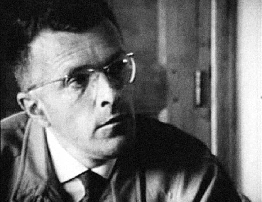
Gilbert Simondon (1924-1989). Photo by LeMonde.
This is a short opinion article to share some notes on the book by the French philosopher Gilbert Simondon called “On the Mode of Existence of Technical Objects” (Du mode d’existence des objets techniques) from 1958. Despite his significant contributions, Simondon still (and incredibly) remains relatively unknown, and it seems to me that this is partly due to the delayed translation of his works. I realized recently that his philosophy of technology aligns very well with an actionable understanding of AI/ML. His insights illuminated a lot for me on how we should approach modern technology and what cultural and societal changes are needed to view AI as an evolving entity that can be harmonised with human needs. This perspective offers an alternative to the current cultural polarization between technophilia and technophobia, which often leads to alienation and misoneism. I think that this work from 1958 provides more enlightening and actionable insights than many contemporary discussions of AI and machine learning, which often prioritise media attention over public education. Simondon’s book is very dense and it was very difficult to read (I found it more difficult than Heidegger’s work on philosophy of technology), so in my quest to simplify it, I might be guilty of simplism in some cases.
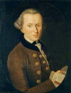
Portrait of Immanuel Kant by Johann Gottlieb Becker, 1768.
One of the most interesting, but also obscure and difficult parts of Kant’s critique is schematism. Every time I reflect on generalisation in Machine Learning and how concepts should be grounded, it always leads to the same central problem of schematism. Friedrich H. Jacobi said that schematism was “the most wonderful and most mysterious of all unfathomable mysteries and wonders …” [1], and Schopenhauer also said that it was “famous for its profound darkness, because nobody has yet been able to make sense of it” [1].
It is very rewarding, however, to realize that it is impossible to read Kant without relating much of his revolutionary philosophy to the difficult problems we are facing (and had always been) in AI, especially regarding generalisation. The first edition of the Critique of Pure Reason (CPR) was published more than 240 years ago, therefore historical context is often required to understand Kant’s writing, and to make things worse there is a lot of debate and lack of consensus among Kant’s scholars, however, even with these difficulties, it is still one of the most relevant and worth reading works of philosophy today.
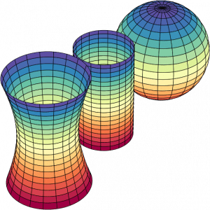
Different gaussian curvature surfaces. Image by Nicoguaro.
We are so used to Euclidean geometry that we often overlook the significance of curved geometries and the methods for measuring things that don’t reside on orthonormal bases. Just as understanding physics and the curvature of spacetime requires Riemannian geometry, I believe a profound comprehension of Machine Learning (ML) and data is also not possible without it. There is an increasing body of research that integrates differential geometry into ML. Unfortunately, the term “geometric deep learning” has predominantly become associated with graphs. However, modern geometry offers much more than just graph-related applications in ML.
I was reading the excellent article from Sander Dieleman about different perspectives on diffusion, so I thought it would be cool to try to contribute a bit with a new perspective.
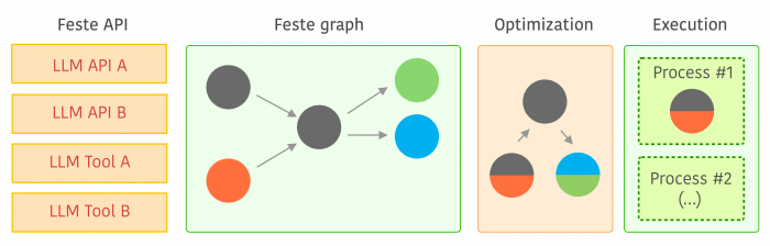
I just released Feste, a free and open-source framework with a permissive license that allows scalable composition of NLP tasks using a graph execution model that is optimized and executed by specialized schedulers. The main idea behind Feste is that it builds a graph of execution instead of executing tasks immediately, this graph allows Feste to optimize and parallelize it. One main example of optimization is when we have multiple calls to the same backend (e.g. same API), Feste automatically fuses these calls into a single one and therefore it batches the call to reduce latency and improve backend inference leverage of GPU vectorization. Feste also executes tasks that can be done in parallel in different processes, so the user doesn’t have to care about parallelization, especially when there are multiple frameworks using different concurrency strategies.
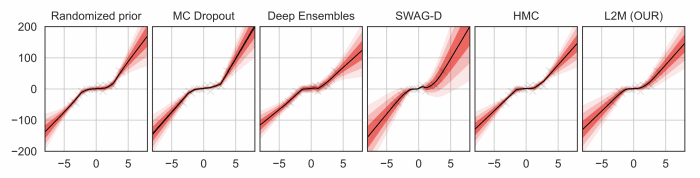
Uncertainty quantification for deep neural networks has recently evolved through many techniques. In this work, we revisit Laplace approximation, a classical approach for posterior approximation that is computationally attractive. However, instead of computing the curvature matrix, we show that, under some regularity conditions, the Laplace approximation can be easily constructed using the gradient second moment. This quantity is already estimated by many exponential moving average variants of Adagrad such as Adam and RMSprop, but is traditionally discarded after training. We show that our method (L2M) does not require changes in models or optimization, can be implemented in a few lines of code to yield reasonable results, and it does not require any extra computational steps besides what is already being computed by optimizers, without introducing any new hyperparameter. We hope our method can open new research directions on using quantities already computed by optimizers for uncertainty estimation in deep neural networks.
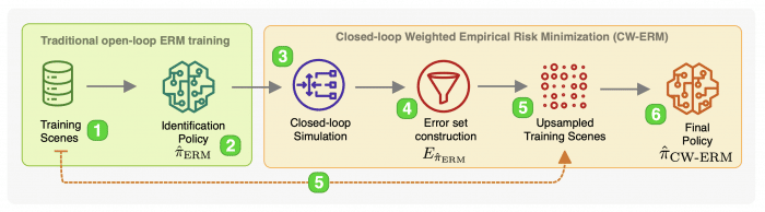
The imitation learning of self-driving vehicle policies through behavioral cloning is often carried out in an open-loop fashion, ignoring the effect of actions to future states. Training such policies purely with Empirical Risk Minimization (ERM) can be detrimental to real-world performance, as it biases policy networks towards matching only open-loop behavior, showing poor results when evaluated in closed-loop. In this work, we develop an efficient and simple-to-implement principle called Closed-loop Weighted Empirical Risk Minimization (CW-ERM), in which a closed-loop evaluation procedure is first used to identify training data samples that are important for practical driving performance and then we these samples to help debias the policy network. We evaluate CW-ERM in a challenging urban driving dataset and show that this procedure yields a significant reduction in collisions as well as other non-differentiable closed-loop metrics.
SafePathNet: Safe Real-World Autonomous Driving by Learning to Predict and Plan with a Mixture of Experts
The goal of autonomous vehicles is to navigate public roads safely and comfortably. To enforce safety, traditional planning approaches rely on handcrafted rules to generate trajectories. Machine learning-based systems, on the other hand, scale with data and are able to learn more complex behaviors. However, they often ignore that agents and self-driving vehicle trajectory distributions can be leveraged to improve safety. In this paper, we propose modeling a distribution over multiple future trajectories for both the self-driving vehicle and other road agents, using a unified neural network architecture for prediction and planning. During inference, we select the planning trajectory that minimizes a cost taking into account safety and the predicted probabilities. Our approach does not depend on any rule-based planners for trajectory generation or optimization, improves with more training data and is simple to implement. We extensively evaluate our method through a realistic simulator and show that the predicted trajectory distribution corresponds to different driving profiles. We also successfully deploy it on a self-driving vehicle on urban public roads, confirming that it drives safely without compromising comfort.
In 2009 I started playing with LLVM for some projects (data structure jit, for genetic programming, jit for tensorflow graphs, etc), and in these projects I realized how powerful LLVM design was at the time (and still is): using an elegant IR (intermediate representation) with an user-facing API and modularized front-ends and backends with plenty of transformation and optimization passes. Nowadays, LLVM is the main engine behind many compilers and JIT compilation and where most of the modern developments in compilers is happening.
On a related note, PyTorch is doing an amazing job of exposing more of the torch tracing system and its IR and graphs, not to mention their work on recent fusers and TorchDynamo. In this context, I was doing a small test to re-implement Shine, but using ATen ops for tensors and realized that there were not many educative tutorials on how to use LLVM to JIT PyTorch graphs, so this is a quick series (if time helps there will be more following posts) on how to use LLVM (python bindings) to go from PyTorch graphs (as traced by torch.fx) to LLVM IR and native code.
Detour – PyTorch NNC (Neural Net Compiler)
PyTorch itself also has a compiler that uses LLVM to generate native code for subgraphs that the fuser identifies. This is also called NNC (Neural Net Compiler) or Tensor Expressions (TE) as well, you can read more about them here in the C++ API tutorial. One thing to note though is that default binaries you get from PyTorch do not come linked to the LLVM libraries, so you need to compile it by yourself and enable LLVM backend, otherwise it won’t use LLVM to do the JIT compilation/optimization of the subgraphs. Let’s take a look at it first before starting our tutorial
This website uses cookies to improve your experience. We'll assume you're ok with this, but you can opt-out if you wish. Cookie settingsACCEPT
Privacy & Cookies Policy
Privacy Overview
This website uses cookies to improve your experience while you navigate through the website. Out of these cookies, the cookies that are categorized as necessary are stored on your browser as they are essential for the working of basic functionalities of the website. We also use third-party cookies that help us analyze and understand how you use this website. These cookies will be stored in your browser only with your consent. You also have the option to opt-out of these cookies. But opting out of some of these cookies may have an effect on your browsing experience.
Necessary cookies are absolutely essential for the website to function properly. This category only includes cookies that ensures basic functionalities and security features of the website. These cookies do not store any personal information.
Any cookies that may not be particularly necessary for the website to function and is used specifically to collect user personal data via analytics, ads, other embedded contents are termed as non-necessary cookies. It is mandatory to procure user consent prior to running these cookies on your website.