If you are following some Machine Learning news, you certainly saw the work done by Ryan Dahl on Automatic Colorization (Hacker News comments, Reddit comments). This amazing work uses pixel hypercolumn information extracted from the VGG-16 network in order to colorize images. Samim also used the network to process Black & White video frames and produced the amazing video below:

https://www.youtube.com/watch?v=_MJU8VK2PI4

Colorizing Black&White Movies with Neural Networks (video by Samim, network by Ryan)

But how does this hypercolumns works ? How to extract them to use on such variety of pixel classification problems ? The main idea of this post is to use the VGG-16 pre-trained network together with Keras and Scikit-Learn in order to extract the pixel hypercolumns and take a superficial look at the information present on it. I’m writing this because I haven’t found anything in Python to do that and this may be really useful for others working on pixel classification, segmentation, etc.

Hypercolumns

Many algorithms using features from CNNs (Convolutional Neural Networks) usually use the last FC (fully-connected) layer features in order to extract information about certain input. However, the information in the last FC layer may be too coarse spatially to allow precise localization (due to sequences of maxpooling, etc.), on the other side, the first layers may be spatially precise but will lack semantic information. To get the best of both worlds, the authors of the hypercolumn paper define the hypercolumn of a pixel as the vector of activations of all CNN units “above” that pixel.

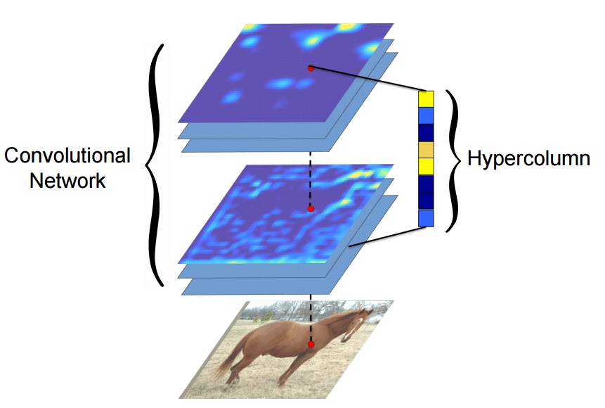
The first step on the extraction of the hypercolumns is to feed the image into the CNN (Convolutional Neural Network) and extract the feature map activations for each location of the image. The tricky part is when the feature maps are smaller than the input image, for instance after a pooling operation, the authors of the paper then do a bilinear upsampling of the feature map in order to keep the feature maps on the same size of the input. There are also the issue with the FC (fully-connected) layers, because you can’t isolate units semantically tied only to one pixel of the image, so the FC activations are seen as 1×1 feature maps, which means that all locations shares the same information regarding the FC part of the hypercolumn. All these activations are then concatenated to create the hypercolumn. For instance, if we take the VGG-16 architecture to use only the first 2 convolutional layers after the max pooling operations, we will have a hypercolumn with the size of:

64 filters (first conv layer before pooling)

+

128 filters (second conv layer before pooling ) = 192 features

This means that each pixel of the image will have a 192-dimension hypercolumn vector. This hypercolumn is really interesting because it will contain information about the first layers (where we have a lot of spatial information but little semantic) and also information about the final layers (with little spatial information and lots of semantics). Thus this hypercolumn will certainly help in a lot of pixel classification tasks such as the one mentioned earlier of automatic colorization, because each location hypercolumn carries the information about what this pixel semantically and spatially represents. This is also very helpful on segmentation tasks (you can see more about that on the original paper introducing the hypercolumn concept).

Everything sounds cool, but how do we extract hypercolumns in practice ?

VGG-16

Before being able to extract the hypercolumns, we’ll setup the VGG-16 pre-trained network, because you know, the price of a good GPU (I can’t even imagine many of them) here in Brazil is very expensive and I don’t want to sell my kidney to buy a GPU.

To setup a pretrained VGG-16 network on Keras, you’ll need to download the weights file from here (vgg16_weights.h5 file with approximately 500MB) and then setup the architecture and load the downloaded weights using Keras (more information about the weights file and architecture here):

from matplotlib import pyplot as plt

import theano
import cv2
import numpy as np
import scipy as sp

from keras.models import Sequential
from keras.layers.core import Flatten, Dense, Dropout
from keras.layers.convolutional import Convolution2D, MaxPooling2D
from keras.layers.convolutional import ZeroPadding2D
from keras.optimizers import SGD

from sklearn.manifold import TSNE
from sklearn import manifold
from sklearn import cluster
from sklearn.preprocessing import StandardScaler

def VGG_16(weights_path=None):
    model = Sequential()
    model.add(ZeroPadding2D((1,1),input_shape=(3,224,224)))
    model.add(Convolution2D(64, 3, 3, activation='relu'))
    model.add(ZeroPadding2D((1,1)))
    model.add(Convolution2D(64, 3, 3, activation='relu'))
    model.add(MaxPooling2D((2,2), stride=(2,2)))

    model.add(ZeroPadding2D((1,1)))
    model.add(Convolution2D(128, 3, 3, activation='relu'))
    model.add(ZeroPadding2D((1,1)))
    model.add(Convolution2D(128, 3, 3, activation='relu'))
    model.add(MaxPooling2D((2,2), stride=(2,2)))

    model.add(ZeroPadding2D((1,1)))
    model.add(Convolution2D(256, 3, 3, activation='relu'))
    model.add(ZeroPadding2D((1,1)))
    model.add(Convolution2D(256, 3, 3, activation='relu'))
    model.add(ZeroPadding2D((1,1)))
    model.add(Convolution2D(256, 3, 3, activation='relu'))
    model.add(MaxPooling2D((2,2), stride=(2,2)))

    model.add(ZeroPadding2D((1,1)))
    model.add(Convolution2D(512, 3, 3, activation='relu'))
    model.add(ZeroPadding2D((1,1)))
    model.add(Convolution2D(512, 3, 3, activation='relu'))
    model.add(ZeroPadding2D((1,1)))
    model.add(Convolution2D(512, 3, 3, activation='relu'))
    model.add(MaxPooling2D((2,2), stride=(2,2)))

    model.add(ZeroPadding2D((1,1)))
    model.add(Convolution2D(512, 3, 3, activation='relu'))
    model.add(ZeroPadding2D((1,1)))
    model.add(Convolution2D(512, 3, 3, activation='relu'))
    model.add(ZeroPadding2D((1,1)))
    model.add(Convolution2D(512, 3, 3, activation='relu'))
    model.add(MaxPooling2D((2,2), stride=(2,2)))

    model.add(Flatten())
    model.add(Dense(4096, activation='relu'))
    model.add(Dropout(0.5))
    model.add(Dense(4096, activation='relu'))
    model.add(Dropout(0.5))
    model.add(Dense(1000, activation='softmax'))

    if weights_path:
        model.load_weights(weights_path)

    return model

As you can see, this is a very simple code to declare the VGG16 architecture and load the pre-trained weights (together with Python imports for the required packages). After that we’ll compile the Keras model:

model = VGG_16('vgg16_weights.h5')
sgd = SGD(lr=0.1, decay=1e-6, momentum=0.9, nesterov=True)
model.compile(optimizer=sgd, loss='categorical_crossentropy')

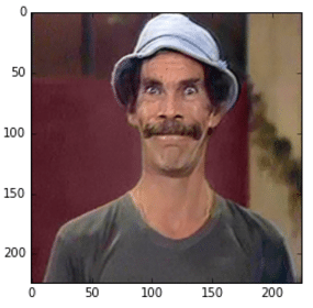
Now let’s test the network using an image:

im_original = cv2.resize(cv2.imread('madruga.jpg'), (224, 224))
im = im_original.transpose((2,0,1))
im = np.expand_dims(im, axis=0)
im_converted = cv2.cvtColor(im_original, cv2.COLOR_BGR2RGB)
plt.imshow(im_converted)

Image used

As we can see, we loaded the image, fixed the axes and then we can now feed the image into the VGG-16 to get the predictions:

out = model.predict(im)
plt.plot(out.ravel())

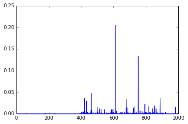
As you can see, these are the final activations of the softmax layer, the class with the “jersey, T-shirt, tee shirt” category.

Extracting arbitrary feature maps

Now, to extract the feature map activations, we’ll have to being able to extract feature maps from arbitrary convolutional layers of the network. We can do that by compiling a Theano function using the get_output() method of Keras, like in the example below:

get_feature = theano.function([model.layers[0].input], model.layers[3].get_output(train=False), allow_input_downcast=False)
feat = get_feature(im)
plt.imshow(feat[0][2])

Feature Map

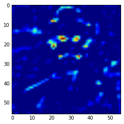
In the example above, I’m compiling a Theano function to get the 3 layer (a convolutional layer) feature map and then showing only the 3rd feature map. Here we can see the intensity of the activations. If we get feature maps of the activations from the final layers, we can see that the extracted features are more abstract, like eyes, etc. Look at this example below from the 15th convolutional layer:

get_feature = theano.function([model.layers[0].input], model.layers[15].get_output(train=False), allow_input_downcast=False)
feat = get_feature(im)
plt.imshow(feat[0][13])

More semantic feature maps.

As you can see, this second feature map is extracting more abstract features. And you can also note that the image seems to be more stretched when compared with the feature we saw earlier, that is because the the first feature maps has 224×224 size and this one has 56×56 due to the downscaling operations of the layers before the convolutional layer, and that is why we lose a lot of spatial information.

Extracting hypercolumns

Now finally let’s extract the hypercolumns of arbitrary set of layers. To do that, we will define a function to extract these hypercolumns:

def extract_hypercolumn(model, layer_indexes, instance):
    layers = [model.layers[li].get_output(train=False) for li in layer_indexes]
    get_feature = theano.function([model.layers[0].input], layers,
                                  allow_input_downcast=False)
    feature_maps = get_feature(instance)
    hypercolumns = []
    for convmap in feature_maps:
        for fmap in convmap[0]:
            upscaled = sp.misc.imresize(fmap, size=(224, 224),
                                        mode="F", interp='bilinear')
            hypercolumns.append(upscaled)

    return np.asarray(hypercolumns)

As we can see, this function will expect three parameters: the model itself, an list of layer indexes that will be used to extract the hypercolumn features and an image instance that will be used to extract the hypercolumns. Let’s now test the hypercolumn extraction for the first 2 convolutional layers:

layers_extract = [3, 8]
hc = extract_hypercolumn(model, layers_extract, im)

That’s it, we extracted the hypercolumn vectors for each pixel. The shape of this “hc” variable is: (192L, 224L, 224L), which means that we have a 192-dimensional hypercolumn for each one of the 224×224 pixel (a total of 50176 pixels with 192 hypercolumn feature each).

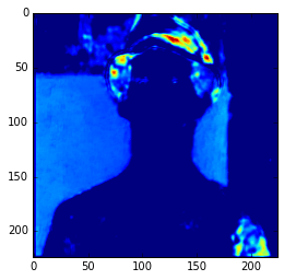
Let’s plot the average of the hypercolumns activations for each pixel:

ave = np.average(hc.transpose(1, 2, 0), axis=2)
plt.imshow(ave)

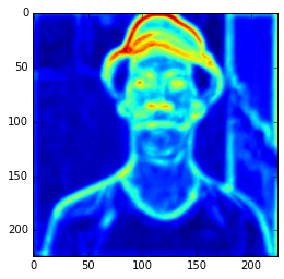
Ad you can see, those first hypercolumn activations are all looking like edge detectors, let’s see how these hypercolumns looks like for the layers 22 and 29:

layers_extract = [22, 29]
hc = extract_hypercolumn(model, layers_extract, im)
ave = np.average(hc.transpose(1, 2, 0), axis=2)
plt.imshow(ave)

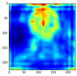
As we can see now, the features are really more abstract and semantically interesting but with spatial information a little fuzzy.

Remember that you can extract the hypercolumns using all the initial layers and also the final layers, including the FC layers. Here I’m extracting them separately to show how they differ in the visualization plots.

Simple hypercolumn pixel clustering

Now, you can do a lot of things, you can use these hypercolumns to classify pixels for some task, to do automatic pixel colorization, segmentation, etc. What I’m going to do here just as an experiment, is to use the hypercolumns (from the VGG-16 layers 3, 8, 15, 22, 29) and then cluster it using KMeans with 2 clusters:

m = hc.transpose(1,2,0).reshape(50176, -1)
kmeans = cluster.KMeans(n_clusters=2, max_iter=300, n_jobs=5, precompute_distances=True)
cluster_labels = kmeans .fit_predict(m)

imcluster = np.zeros((224,224))
imcluster = imcluster.reshape((224*224,))
imcluster = cluster_labels

plt.imshow(imcluster.reshape(224, 224), cmap="hot")

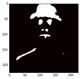
Now you can imagine how useful hypercolumns can be to tasks like keypoints extraction, segmentation, etc. It’s a very elegant, simple and useful concept.

I hope you liked it !

– Christian S. Perone