I was taking a look at the proposal N2765 (user-defined literals) already implemented on the development snapshots of the GCC 4.7 and I was thinking in how user-defined literals can be used to create some interesting and sometimes strange constructions.
Introduction to user-defined literals
C++03 has some literals, like the “f” in “12.2f” that converts the double value to float. The problem is that these literals aren’t very flexible since they’re pretty fixed, so you can’t change them or create new ones. To overcome this situation, C++11 introduced the concept of “user-defined literals” that will give to the user, the ability to create new custom literal modifiers. The new user-defined literals can create either built-in types (e.g. int) or user-define types (e.g. classes), and the fact that they could be very useful is an effect that they can return objects instead of only primitives.
… in the case of a literal string. The OutputType is anything you want (object or primitive), the “_suffix” is the name of the literal modifier, isn’t required to use the underline in front of it, but if you don’t use you’ll get some warnings telling you that suffixes not preceded by the underline are reserved for future standardization.
Examples
Kmh to Mph converter
[enlighter lang=”C++” escaped=”true” lines=”1000″]
// stupid converter class
class Converter
{
public:
Converter(double kmph) : m_kmph(kmph) {};
~Converter() {};
int main(void)
{
std::cout << “Converter: ” << (80kmph).to_mph() << std::endl;
// note that I’m using parenthesis in order to
// be able to call the ‘to_mph’ method
return 0;
}
[/ccb]
Note that the literal for for numeric types should be either long double (for floating point literals) or unsigned long long (for integral literals). There is no signed type, because a signed literal is parsed as an expression with a sign as unary prefix and the unsigned number part.
int main(void)
{
std::cout << "convert me to a string"s.length() << std::endl;
// here you don't need the parenthesis, note that the
// c-string was automagically converted to std::string
return 0;
}
[/ccb]
This post is a continuation of the first part where we started to learn the theory and practice about text feature extraction and vector space model representation. I really recommend you to read the first part of the post series in order to follow this second post.
Since a lot of people liked the first part of this tutorial, this second part is a little longer than the first.
Introduction
In the first post, we learned how to use the term-frequency to represent textual information in the vector space. However, the main problem with the term-frequency approach is that it scales up frequent terms and scales down rare terms which are empirically more informative than the high frequency terms. The basic intuition is that a term that occurs frequently in many documents is not a good discriminator, and really makes sense (at least in many experimental tests); the important question here is: why would you, in a classification problem for instance, emphasize a term which is almost present in the entire corpus of your documents ?
The tf-idf weight comes to solve this problem. What tf-idf gives is how important is a word to a document in a collection, and that’s why tf-idf incorporates local and global parameters, because it takes in consideration not only the isolated term but also the term within the document collection. What tf-idf then does to solve that problem, is to scale down the frequent terms while scaling up the rare terms; a term that occurs 10 times more than another isn’t 10 times more important than it, that’s why tf-idf uses the logarithmic scale to do that.
But let’s go back to our definition of the which is actually the term count of the term in the document . The use of this simple term frequency could lead us to problems like keyword spamming, which is when we have a repeated term in a document with the purpose of improving its ranking on an IR (Information Retrieval) system or even create a bias towards long documents, making them look more important than they are just because of the high frequency of the term in the document.
To overcome this problem, the term frequency of a document on a vector space is usually also normalized. Let’s see how we normalize this vector.
Vector normalization
Suppose we are going to normalize the term-frequency vector that we have calculated in the first part of this tutorial. The document from the first part of this tutorial had this textual representation:
d4: We can see the shining sun, the bright sun.
And the vector space representation using the non-normalized term-frequency of that document was:
To normalize the vector, is the same as calculating the Unit Vector of the vector, and they are denoted using the “hat” notation: . The definition of the unit vector of a vector is:
Where the is the unit vector, or the normalized vector, the is the vector going to be normalized and the is the norm (magnitude, length) of the vector in the space (don’t worry, I’m going to explain it all).
The unit vector is actually nothing more than a normalized version of the vector, is a vector which the length is 1.
The normalization process (Source: http://processing.org/learning/pvector/)
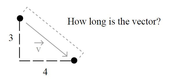
But the important question here is how the length of the vector is calculated and to understand this, you must understand the motivation of the spaces, also called Lebesgue spaces.
Lebesgue spaces
How long is this vector ? (Source: Source: http://processing.org/learning/pvector/)
Usually, the length of a vector is calculated using the Euclidean norm – a norm is a function that assigns a strictly positive length or size to all vectors in a vector space -, which is defined by:
(Source: http://processing.org/learning/pvector/)
But this isn’t the only way to define length, and that’s why you see (sometimes) a number together with the norm notation, like in . That’s because it could be generalized as:
and simplified as:
So when you read about a L2-norm, you’re reading about the Euclidean norm, a norm with , the most common norm used to measure the length of a vector, typically called “magnitude”; actually, when you have an unqualified length measure (without the number), you have the L2-norm (Euclidean norm).
When you read about a L1-norm, you’re reading about the norm with , defined as:
Which is nothing more than a simple sum of the components of the vector, also known as Taxicab distance, also called Manhattan distance.
Taxicab geometry versus Euclidean distance: In taxicab geometry all three pictured lines have the same length (12) for the same route. In Euclidean geometry, the green line has length , and is the unique shortest path.
Source: Wikipedia :: Taxicab Geometry
Note that you can also use any norm to normalize the vector, but we’re going to use the most common norm, the L2-Norm, which is also the default in the 0.9 release of the scikits.learn. You can also find papers comparing the performance of the two approaches among other methods to normalize the document vector, actually you can use any other method, but you have to be concise, once you’ve used a norm, you have to use it for the whole process directly involving the norm (a unit vector that used a L1-norm isn’t going to have the length 1 if you’re going to take its L2-norm later).
Back to vector normalization
Now that you know what the vector normalization process is, we can try a concrete example, the process of using the L2-norm (we’ll use the right terms now) to normalize our vector in order to get its unit vector . To do that, we’ll simple plug it into the definition of the unit vector to evaluate it:
And that is it ! Our normalized vector has now a L2-norm .
Note that here we have normalized our term frequency document vector, but later we’re going to do that after the calculation of the tf-idf.
The term frequency – inverse document frequency (tf-idf) weight
Now you have understood how the vector normalization works in theory and practice, let’s continue our tutorial. Suppose you have the following documents in your collection (taken from the first part of tutorial):
Train Document Set:

d1: The sky is blue.
d2: The sun is bright.

Test Document Set:

d3: The sun in the sky is bright.
d4: We can see the shining sun, the bright sun.
Your document space can be defined then as where is the number of documents in your corpus, and in our case as and . The cardinality of our document space is defined by and , since we have only 2 two documents for training and testing, but they obviously don’t need to have the same cardinality.
Let’s see now, how idf (inverse document frequency) is then defined:
where is the number of documents where the term appears, when the term-frequency function satisfies , we’re only adding 1 into the formula to avoid zero-division.
The formula for the tf-idf is then:
and this formula has an important consequence: a high weight of the tf-idf calculation is reached when you have a high term frequency (tf) in the given document (local parameter) and a low document frequency of the term in the whole collection (global parameter).
Now let’s calculate the idf for each feature present in the feature matrix with the term frequency we have calculated in the first tutorial:
Since we have 4 features, we have to calculate , , , :
These idf weights can be represented by a vector as:
Now that we have our matrix with the term frequency () and the vector representing the idf for each feature of our matrix (), we can calculate our tf-idf weights. What we have to do is a simple multiplication of each column of the matrix with the respective vector dimension. To do that, we can create a square diagonal matrix called with both the vertical and horizontal dimensions equal to the vector dimension:
and then multiply it to the term frequency matrix, so the final result can be defined then as:
Please note that the matrix multiplication isn’t commutative, the result of will be different than the result of the , and this is why the is on the right side of the multiplication, to accomplish the desired effect of multiplying each idf value to its corresponding feature:
Let’s see now a concrete example of this multiplication:
And finally, we can apply our L2 normalization process to the matrix. Please note that this normalization is “row-wise” because we’re going to handle each row of the matrix as a separated vector to be normalized, and not the matrix as a whole:
And that is our pretty normalized tf-idf weight of our testing document set, which is actually a collection of unit vectors. If you take the L2-norm of each row of the matrix, you’ll see that they all have a L2-norm of 1.
Now the section you were waiting for ! In this section I’ll use Python to show each step of the tf-idf calculation using the Scikit.learn feature extraction module.
The first step is to create our training and testing document set and computing the term frequency matrix:
from sklearn.feature_extraction.text import CountVectorizer

train_set = ("The sky is blue.", "The sun is bright.")
test_set = ("The sun in the sky is bright.",
"We can see the shining sun, the bright sun.")

count_vectorizer = CountVectorizer()
count_vectorizer.fit_transform(train_set)
print "Vocabulary:", count_vectorizer.vocabulary

# Vocabulary: {'blue': 0, 'sun': 1, 'bright': 2, 'sky': 3}

freq_term_matrix = count_vectorizer.transform(test_set)
print freq_term_matrix.todense()

#[[0 1 1 1]
#[0 2 1 0]]
Now that we have the frequency term matrix (called freq_term_matrix), we can instantiate the TfidfTransformer, which is going to be responsible to calculate the tf-idf weights for our term frequency matrix:
Note that I’ve specified the norm as L2, this is optional (actually the default is L2-norm), but I’ve added the parameter to make it explicit to you that it it’s going to use the L2-norm. Also note that you can see the calculated idf weight by accessing the internal attribute called idf_. Now that fit() method has calculated the idf for the matrix, let’s transform the freq_term_matrix to the tf-idf weight matrix:
And that is it, the tf_idf_matrix is actually our previous matrix. You can accomplish the same effect by using the Vectorizer class of the Scikit.learn which is a vectorizer that automatically combines the CountVectorizer and the TfidfTransformer to you. See this example to know how to use it for the text classification process.
I really hope you liked the post, I tried to make it simple as possible even for people without the required mathematical background of linear algebra, etc. In the next Machine Learning post I’m expecting to show how you can use the tf-idf to calculate the cosine similarity.
If you liked it, feel free to comment and make suggestions, corrections, etc.
In information retrieval or text mining, the term frequency – inverse document frequency (also called tf-idf), is a well know method to evaluate how important is a word in a document. tf-idf are is a very interesting way to convert the textual representation of information into a Vector Space Model (VSM), or into sparse features, we’ll discuss more about it later, but first, let’s try to understand what is tf-idf and the VSM.
VSM has a very confusing past, see for example the paper The most influential paper Gerard Salton Never Wrote that explains the history behind the ghost cited paper which in fact never existed; in sum, VSM is an algebraic model representing textual information as a vector, the components of this vector could represent the importance of a term (tf–idf) or even the absence or presence (Bag of Words) of it in a document; it is important to note that the classical VSM proposed by Salton incorporates local and global parameters/information (in a sense that it uses both the isolated term being analyzed as well the entire collection of documents). VSM, interpreted in a lato sensu, is a space where text is represented as a vector of numbers instead of its original string textual representation; the VSM represents the features extracted from the document.
Let’s try to mathematically define the VSM and tf-idf together with concrete examples, for the concrete examples I’ll be using Python (as well the amazing scikits.learn Python module).
Going to the vector space
The first step in modeling the document into a vector space is to create a dictionary of terms present in documents. To do that, you can simple select all terms from the document and convert it to a dimension in the vector space, but we know that there are some kind of words (stop words) that are present in almost all documents, and what we’re doing is extracting important features from documents, features do identify them among other similar documents, so using terms like “the, is, at, on”, etc.. isn’t going to help us, so in the information extraction, we’ll just ignore them.
Let’s take the documents below to define our (stupid) document space:
Train Document Set:

d1: The sky is blue.
d2: The sun is bright.

Test Document Set:

d3: The sun in the sky is bright.
d4: We can see the shining sun, the bright sun.
Now, what we have to do is to create a index vocabulary (dictionary) of the words of the train document set, using the documents and from the document set, we’ll have the following index vocabulary denoted as where the is the term:
Note that the terms like “is” and “the” were ignored as cited before. Now that we have an index vocabulary, we can convert the test document set into a vector space where each term of the vector is indexed as our index vocabulary, so the first term of the vector represents the “blue” term of our vocabulary, the second represents “sun” and so on. Now, we’re going to use the term-frequency to represent each term in our vector space; the term-frequency is nothing more than a measure of how many times the terms present in our vocabulary are present in the documents or , we define the term-frequency as a couting function:
where the is a simple function defined as:
So, what the returns is how many times is the term is present in the document . An example of this, could be since we have only two occurrences of the term “sun” in the document . Now you understood how the term-frequency works, we can go on into the creation of the document vector, which is represented by:
Each dimension of the document vector is represented by the term of the vocabulary, for example, the represents the frequency-term of the term 1 or (which is our “blue” term of the vocabulary) in the document .
Let’s now show a concrete example of how the documents and are represented as vectors:
which evaluates to:
As you can see, since the documents and are:
d3: The sun in the sky is bright.
d4: We can see the shining sun, the bright sun.
The resulting vector shows that we have, in order, 0 occurrences of the term “blue”, 1 occurrence of the term “sun”, and so on. In the , we have 0 occurences of the term “blue”, 2 occurrences of the term “sun”, etc.
But wait, since we have a collection of documents, now represented by vectors, we can represent them as a matrix with shape, where is the cardinality of the document space, or how many documents we have and the is the number of features, in our case represented by the vocabulary size. An example of the matrix representation of the vectors described above is:
As you may have noted, these matrices representing the term frequencies tend to be very sparse (with majority of terms zeroed), and that’s why you’ll see a common representation of these matrix as sparse matrices.
Since we know the theory behind the term frequency and the vector space conversion, let’s show how easy is to do that using the amazing scikit.learn Python module.
Scikit.learn comes with lots of examples as well real-life interesting datasets you can use and also some helper functions to download 18k newsgroups posts for instance.
Since we already defined our small train/test dataset before, let’s use them to define the dataset in a way that scikit.learn can use:
train_set = ("The sky is blue.", "The sun is bright.")
test_set = ("The sun in the sky is bright.",
    "We can see the shining sun, the bright sun.")
In scikit.learn, what we have presented as the term-frequency, is called CountVectorizer, so we need to import it and create a news instance:
from sklearn.feature_extraction.text import CountVectorizer
vectorizer = CountVectorizer()
The CountVectorizer already uses as default “analyzer” called WordNGramAnalyzer, which is responsible to convert the text to lowercase, accents removal, token extraction, filter stop words, etc… you can see more information by printing the class information:
Note that the sparse matrix created called smatrix is a Scipy sparse matrix with elements stored in a Coordinate format. But you can convert it into a dense format:
Note that the sparse matrix created is the same matrix we cited earlier in this post, which represents the two document vectors and .
We’ll see in the next post how we define the idf (inverse document frequency) instead of the simple term-frequency, as well how logarithmic scale is used to adjust the measurement of term frequencies according to its importance, and how we can use it to classify documents using some of the well-know machine learning approaches.
I hope you liked this post, and if you really liked, leave a comment so I’ll able to know if there are enough people interested in these series of posts in Machine Learning topics.
21 Sep 11 – fixed some typos and the vector notation 22 Sep 11 – fixed import of sklearn according to the new 0.9 release and added the environment section 02 Oct 11 – fixed Latex math typos 18 Oct 11 – added link to the second part of the tutorial series 04 Mar 11 – Fixed formatting issues
What I’ve built to consider these questions is an interactive robotic painting machine that uses artificial intelligence to paint its own body of work and to make its own decisions. While doing so, it listens to its environment and considers what it hears as input into the painting process. In the absence of someone or something else making sound in its presence, the machine, like many artists, listens to itself. But when it does hear others, it changes what it does just as we subtly (or not so subtly) are influenced by what others tell us.
An evolutionary computation approach developed by Franklin University’s Esmail Bonakdarian, Ph.D., was used to analyze data from two classical economics experiments. As can be seen in this figure, optimization of the search over subsets of the maximum model proceeds initially at a quick rate and then slowly continues to improve over time until it converges. The top curve (red) shows the optimum value found so far, while the lower, jagged line (green) shows the current average fitness value for the population in each generation.
(…)
Regression analysis has been the traditional tool for finding and establishing statistically significant relationships in research projects, such as for the economics examples Bonakdarian chose. As long as the number of independent variables is relatively small, or the experimenter has a fairly clear idea of the possible underlying relationship, it is feasible to derive the best model using standard software packages and methodologies.
However, Bonakdarian cautioned that if the number of independent variables is large, and there is no intuitive sense about the possible relationship between these variables and the dependent variable, “the experimenter may have to go on an automated ‘fishing expedition’ to discover the important and relevant independent variables.”
I’ve made those slides in March of this year to a training session, I was expecting to get time to update it to cover more features but I wasn’t able to do that yet, so I’m publishing it here for those who are interested in some of the new language features.
A new published paper called “NP-hardness of Deciding Convexity of Quartic Polynomials and Related Problems” brings light (or darkness) into a 20 years-old problem related to the whether or not does exist a polynomial time algorithm that can decide if a multivariate polynomial is globally convex. The answer is: NO.
Convex (top) vs Non Convex (bottom) Functions (Source: MIT News)
From the news article:
For complex functions, finding global minima can be very hard. But it’s a lot easier if you know in advance that the function is convex, meaning that the graph of the function slopes everywhere toward the minimum. Convexity is such a useful property that, in 1992, when a major conference on optimization selected the seven most important outstanding problems in the field, one of them was whether the convexity of an arbitrary polynomial function could be efficiently determined.
Almost 20 years later, researchers in MIT’s Laboratory for Information and Decision Systems have finally answered that question. Unfortunately, the answer, which they reported in May with one paper at the Society for Industrial and Applied Mathematics (SIAM) Conference on Optimization, is no. For an arbitrary polynomial function — that is, a function in which variables are raised to integral exponents, such as 13x4 + 7xy2 + yz — determining whether it’s convex is what’s called NP-hard. That means that the most powerful computers in the world couldn’t provide an answer in a reasonable amount of time.
At the same conference, however, MIT Professor of Electrical Engineering and Computer Science Pablo Parrilo and his graduate student Amir Ali Ahmadi, two of the first paper’s four authors, showed that in many cases, a property that can be determined efficiently, known as sum-of-squares convexity, is a viable substitute for convexity. Moreover, they provide an algorithm for determining whether an arbitrary function has that property.
This website uses cookies to improve your experience. We'll assume you're ok with this, but you can opt-out if you wish. Cookie settingsACCEPT
Privacy & Cookies Policy
Privacy Overview
This website uses cookies to improve your experience while you navigate through the website. Out of these cookies, the cookies that are categorized as necessary are stored on your browser as they are essential for the working of basic functionalities of the website. We also use third-party cookies that help us analyze and understand how you use this website. These cookies will be stored in your browser only with your consent. You also have the option to opt-out of these cookies. But opting out of some of these cookies may have an effect on your browsing experience.
Necessary cookies are absolutely essential for the website to function properly. This category only includes cookies that ensures basic functionalities and security features of the website. These cookies do not store any personal information.
Any cookies that may not be particularly necessary for the website to function and is used specifically to collect user personal data via analytics, ads, other embedded contents are termed as non-necessary cookies. It is mandatory to procure user consent prior to running these cookies on your website.
") which is actually the term count of the term
which is actually the term count of the term  in the document
  . The use of this simple term frequency could lead us to problems like keyword spamming, which is when we have a repeated term in a document with the purpose of improving its ranking on an IR (Information Retrieval) system or even create a bias towards long documents, making them look more important than they are just because of the high frequency of the term in the document.
 that we have calculated in the first part of this tutorial. The document
  from the first part of this tutorial had this textual representation:
")
 . The definition of the unit vector
  is:
is:
 is the norm (magnitude, length) of the vector
  space (don’t worry, I’m going to explain it all).
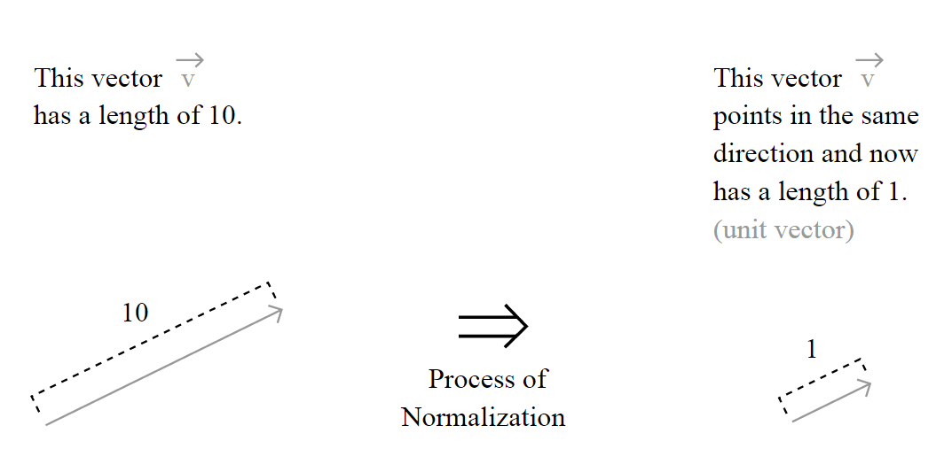
") is calculated using the
is calculated using the 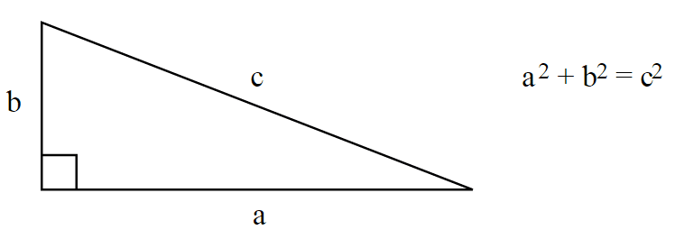

 together with the norm notation, like in
  . That’s because it could be generalized as:
^\frac{1}{p}")
^\frac{1}{p}")
 , the most common norm used to measure the length of a vector, typically called “magnitude”; actually, when you have an unqualified length measure (without the
  , defined as:
")

 , and is the unique shortest path.
 . To do that, we’ll simple plug it into the definition of the unit vector to evaluate it:
}{\sqrt{0^2 + 2^2 + 1^2 + 0^2}} \\ \\ \hat{v_{d_4}} = \frac{(0,2,1,0)}{\sqrt{5}} \\ \\ \small \hat{v_{d_4}} = (0.0, 0.89442719, 0.4472136, 0.0)")
 .
. where
where  is the number of documents in your corpus, and in our case as
  and
and  . The cardinality of our document space is defined by
  and
and  , since we have only 2 two documents for training and testing, but they obviously don’t need to have the same cardinality.
 = \log{\frac{\left|D\right|}{1+\left|\{d : t \in d\}\right|}}")
 is the number of documents where the term
  \neq 0") , we’re only adding 1 into the formula to avoid zero-division.
, we’re only adding 1 into the formula to avoid zero-division. = \mathrm{tf}(t, d) \times \mathrm{idf}(t)")

") ,
, ") ,
, ") ,
, ") :
: = \log{\frac{\left|D\right|}{1+\left|\{d : t_1 \in d\}\right|}} = \log{\frac{2}{1}} = 0.69314718")
 = \log{\frac{\left|D\right|}{1+\left|\{d : t_2 \in d\}\right|}} = \log{\frac{2}{3}} = -0.40546511")
 = \log{\frac{\left|D\right|}{1+\left|\{d : t_3 \in d\}\right|}} = \log{\frac{2}{3}} = -0.40546511")
 = \log{\frac{\left|D\right|}{1+\left|\{d : t_4 \in d\}\right|}} = \log{\frac{2}{2}} = 0.0")
")
 ) and the vector representing the idf for each feature of our matrix (
 ), we can calculate our tf-idf weights. What we have to do is a simple multiplication of each column of the matrix
  with both the vertical and horizontal dimensions equal to the vector

 will be different than the result of the
  , and this is why the
  & \mathrm{tf}(t_2, d_1) & \mathrm{tf}(t_3, d_1) & \mathrm{tf}(t_4, d_1)\\ \mathrm{tf}(t_1, d_2) & \mathrm{tf}(t_2, d_2) & \mathrm{tf}(t_3, d_2) & \mathrm{tf}(t_4, d_2) \end{bmatrix} \times \begin{bmatrix} \mathrm{idf}(t_1) & 0 & 0 & 0\\ 0 & \mathrm{idf}(t_2) & 0 & 0\\ 0 & 0 & \mathrm{idf}(t_3) & 0\\ 0 & 0 & 0 & \mathrm{idf}(t_4) \end{bmatrix} \\ = \begin{bmatrix} \mathrm{tf}(t_1, d_1) \times \mathrm{idf}(t_1) & \mathrm{tf}(t_2, d_1) \times \mathrm{idf}(t_2) & \mathrm{tf}(t_3, d_1) \times \mathrm{idf}(t_3) & \mathrm{tf}(t_4, d_1) \times \mathrm{idf}(t_4)\\ \mathrm{tf}(t_1, d_2) \times \mathrm{idf}(t_1) & \mathrm{tf}(t_2, d_2) \times \mathrm{idf}(t_2) & \mathrm{tf}(t_3, d_2) \times \mathrm{idf}(t_3) & \mathrm{tf}(t_4, d_2) \times \mathrm{idf}(t_4) \end{bmatrix}")

 matrix. Please note that this normalization is “row-wise” because we’re going to handle each row of the matrix as a separated vector to be normalized, and not the matrix as a whole:

 and
and  from the document set, we’ll have the following index vocabulary denoted as
 ") where the
where the  = \begin{cases} 1, & \mbox{if } t\mbox{ is \"blue\"} \\ 2, & \mbox{if } t\mbox{ is \"sun\"} \\ 3, & \mbox{if } t\mbox{ is \"bright\"} \\ 4, & \mbox{if } t\mbox{ is \"sky\"} \\ \end{cases}")
 or
or  = \sum\limits_{x\in d} \mathrm{fr}(x, t)")
") is a simple function defined as:
is a simple function defined as: = \begin{cases} 1, & \mbox{if } x = t \\ 0, & \mbox{otherwise} \\ \end{cases}")
") returns is how many times is the term
returns is how many times is the term  = 2") since we have only two occurrences of the term “sun” in the document
since we have only two occurrences of the term “sun” in the document , \mathrm{tf}(t_2,d_n), \mathrm{tf}(t_3,d_n), \ldots, \mathrm{tf}(t_n,d_n))")
") represents the frequency-term of the term 1 or
represents the frequency-term of the term 1 or  (which is our “blue” term of the vocabulary) in the document
  .
. and
and  are represented as vectors:
, \mathrm{tf}(t_2,d_3), \mathrm{tf}(t_3,d_3), \ldots, \mathrm{tf}(t_n,d_3)) \\ \vec{v_{d_4}} = (\mathrm{tf}(t_1,d_4), \mathrm{tf}(t_2,d_4), \mathrm{tf}(t_3,d_4), \ldots, \mathrm{tf}(t_n,d_4))")
 \\ \vec{v_{d_4}} = (0, 2, 1, 0)")
 shows that we have, in order, 0 occurrences of the term “blue”, 1 occurrence of the term “sun”, and so on. In the
  shape, where
  is the cardinality of the document space, or how many documents we have and the
  is the number of features, in our case represented by the vocabulary size. An example of the matrix representation of the vectors described above is:
") (except because it is zero-indexed).
(except because it is zero-indexed). we cited earlier in this post, which represents the two document vectors


