Diffusion Elites + World Models: surprisingly good, simple and embarrassingly parallel
Introduction
 It is not a secret that Diffusion models have become the workhorses of high-dimensionality generation: start with a Gaussian noise and, through a learned denoising trajectory, you get high-fidelity images, molecular graphs, or robot trajectories that look (uncannily) real. I wrote extensively about diffusion and its connection with the data manifold metric tensor recently as well, so if you are interested please take a look on it.
Now, for many engineering and practical tasks we care less about “looking real” and more about maximising a task-specific score or a reward from a simulator, a chemistry docking metric, a CLIP consistency score, human preference, etc. Even though we can use guidance or do a constrained sampling from the model, we often require differentiable functions for that. Evolution-style search methods (CEM, CMA-ES, etc), however, can shine in that regime, but naively applying them in the raw object space wastes most samples on absurd or invalid candidates and takes a lot of time to converge to a reasonable solution.
I have been experimenting on some personal projects with something that we can call “Diffusion Elites“, which aims to close this gap by letting a pre-trained diffusion model provide the prior and letting an adapted Cross-Entropy Method (CEM) steer the search inside its latent space instead. I found that this works quite well for many domains and it is also an impressively flexible method with a lot to explore (I will talk about some cases later).
To summarize, the method is as simple as the following:
- Draw a population of latent vectors from a Gaussian
- Run one full denoise pass to turn each latent into a structured object
- Score every object with any reward function
- Keep the top-K “elite” latents, refit a new Gaussian to them, and iterate
This five-line loop inherits the robust, gradient-free advantages of evolutionary search while guaranteeing that every candidate lives on the diffusion model’s data manifold. In practice that means fewer wasted evaluations, faster convergence, and dramatically higher-quality solutions for many tasks (e.g. planning, design, etc). In the rest of this post I will unpack the Diffusion Elites in detail, from the algorithm to some coding examples. Diffusion Elites shows that you can explore a diffusion model and turn it into a powerful black box optimizer, it is like doing search on the data manifold itself.
Diffusion Elites
Overview diagram
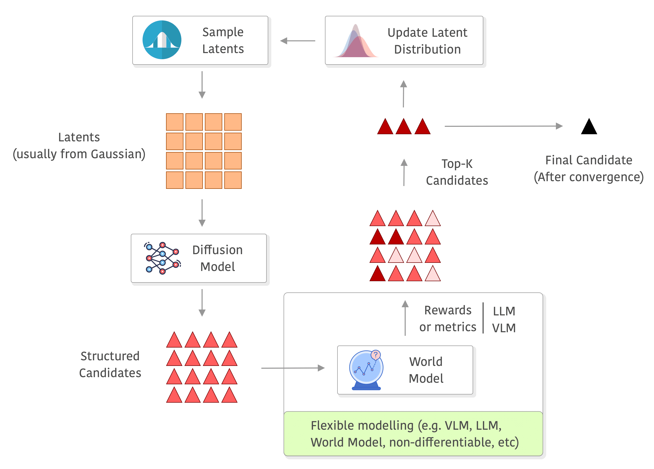
Below you can see a diagram of the process, I added a world model in the rewards to exemplify how you can use a world model and even do roll-outs there without any differentiability requirements, but you can really use anything to compute your rewards (e.g. you can also compute metrics on the outputs of the world model, or use a VLM/LLM as judge or even as world model as well):
Algorithm
The algorithm of Diffusion Elites is described below:
Inputs
\(f:\mathbb{R}^d\!\to\!\mathcal{X}\) — fixed decoder
\(R:\mathcal{X}\!\to\!\mathbb{R}\) — reward function
\(N\in\mathbb{N}\) — population size
\(ρ\in(0,1)\) — elite fraction
\(T\in\mathbb{N}\) — iterations
\(ε>0\) — jitter
Initialise
\(μ_0=\mathbf{0}_d,\;Σ_0=I_d\)
for \(t=0…T-1\) do
▸ Sample \(z_i^{(t)}\sim\mathcal{N}(μ_t,Σ_t)\) for \(i=1…N\)
▸ Decode \(x_i=f(z_i^{(t)})\)
▸ Score \(r_i=R(x_i)\)
▸ Select \(γ_t=\operatorname{quantile}_{1-ρ}\{r_1,…,r_N\}\)
\(E_t=\{z_i^{(t)}:r_i≥γ_t\}\)
▸ Update \(μ_{t+1}=|E_t|^{-1}\!\sum_{z\in E_t}z\)
\(Σ_{t+1}=|E_t|^{-1}\!\sum_{z\in E_t}(z-μ_{t+1})(z-μ_{t+1})^{⊤}+εI_d\)
end for
Output
\(x_\text{best}=\arg\max_{i,t}r_i\)
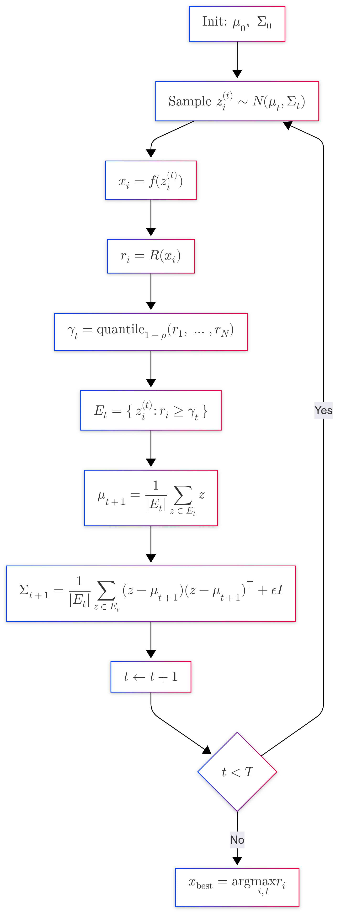
It looks complicated but it is actually quite simple, you just start with a standard Gaussian for the latents, you sample a population with N samples from it \(z_i^{(t)}\sim\mathcal{N}(μ_t,Σ_t)\), then you run your pre-trained Diffusion model \(x_i=f(z_i^{(t)})\) which will get you a sample from the model given the latent \(z_i^{(t)}\), then you calculate your reward \(r_i=R(x_i)\) which can really be anything and doesn’t need to be differentiable as in other approaches doing guidance, then you select a proportion (e.g. 10%) of the top-k individuals, you refit your Gaussian distribution (e.g. using MLE) and keep iterating on that. You can also see a visual diagram of the algorithm below:
If you use a simple diagonal Gaussian, you can fit the algorithm in a few lines of PyTorch code as in the example below, which might help you understand how it looks like:
shape = (batch_size, sample_size)
mu  = torch.zeros((1, sample_size))
std = torch.full_like(mu, 1.0)
min_std = 0.01
n_iters = 10
elite_frac = 0.1  # 10% elite
diffusion = (...) # A pre-trained Diffusion model

elite_size = max(1, int(batch_size * elite_frac))

for it in range(n_iters):
    # 1. sample population
    eps0 = mu + std * torch.randn(shape)

    # 2. decode
    samples = diffusion.sample(shape, eps0, steps=60, eta=0.0)

    # 3. reward and raking
    rewards = reward_function(samples)
    elites = torch.topk(rewards, elite_size, largest=False).indices
    elite_eps = eps0[elites]

    # 4. refit Gaussian
    mu  = elite_eps.mean(dim=0, keepdim=True)
    var = ((elite_eps - mu) ** 2).mean(dim=0, keepdim=True)
    std = torch.sqrt(var + 1e-6).clamp(min=min_std)

    elites = samples[elites]
I haven’t seen this algorithm before being used with a Diffusion model, but I think it is a very interesting and simple algorithm. I saw something similar on Diffusion-ES, which also runs gradient-free search over diffusion samples, but mutates trajectories by partial noising/denoising at every ES generation, while Diffusion Elites (DE) stays in the initial Gaussian latent and uses a clean CEM (Cross-Entropy Method) loop, giving simpler theory as well.
Interesting properties
Now, there are a few interesting properties in this algorithm which I will describe below.
Parallelization
Note that the sampling from either the Gaussian or Diffusion can be done in parallel, they are independent samples and you can run your Diffusion model distributed across how many nodes you want and you can also take leverage of using the largest batch size you can afford too. Also, the reward computation is also easy to distribute, you can compute it on distributed nodes too (just like you did with the Diffusion model too). This makes the method very flexible and amenable to use island models for example, where you evolve populations distributed in islands and can optionally exchange individuals through time. This creates a large distributed search which I think is similar to the approach taken on AlphaEvolve, although they don’t seem to be exchanging individuals across islands.
Highly flexible reward
Note that you don’t have the differentiability requirement for the reward here, you can think about it as a black box. This allows you to do all sorts of things, a few examples include:
- Using a world model in the reward, so for instance, you can do a roll-out in the world model and compute rewards or metrics
- Using any kind of simulator (e.g. physics, fluids, etc) where you will be evaluating your sample afterwards
- If you are generating images, you can use a VLM or even an object detection to make sure it contains some elements you are looking for, kind of a structured guidance that goes beyond prompting
- You can use any LLM to evaluate your sample depending on what your sample is and provide a reward for it
- You can even use preferences here through a reward model, etc
- If you reward tends to be differentiable, you can still use guidance with another non-differentiable reward, there is nothing that would block you from doing this in the algorithm
- The choices are really endless
And as I mentioned above, you can do all of this in parallel, you can easily distributed the reward function computation so you can have very expensive computation there.
Speed-ups
While you are searching during the iteration loop of Diffusion Elites, you don’t have to run too many denoising steps because you are basically ranking samples and you don’t often need a high quality sample for the sake of evaluation, so you can just do a few DDIM steps for example and then do a higher number of steps only for the final samples that you are interested in after convergence, by doing this you are speeding up the inner loop of the denoising on the Diffusion sampling.
Expressive but low-dimensionality search
Latent spaces of modern LDMs (Latent Diffusion Models) are typically 4-8x smaller than pixel/action space, so working on the latent space is much more efficient than working on the structured sample space.
Stay in the manifold
I always like to think about Diffusion as learning the main building block of the metric tensor for the data manifold, so when we work on the latent space of the Diffusion models, we are staying within the realm of the data manifold.
Flexible modelling of the latent distribution
You obviously don’t need to use a Gaussian only for re-fitting the latent distribution, you can start with a standard Gaussian and then later re-fix a mixture, use ensembles, or whatever other option you might want to to consider (there are a lot of papers with many interesting choices for it) that can explore better the latent space at the trade-off of perhaps having more iteration steps needed to converge.
Experiments and visualizations
To help visualize the search for solutions and modelling, I’m going to generate a random dataset of trajectories using a simple kinematic model, then train a Diffusion model on it using a 1D CNN UNet with attention with v-prediction objective and DDIM sampling, so nothing fancy there, just a regular Diffusion model as used for audio signals as well. I used a RTX5090 for the experiments as well as you don’t need a lot of memory for simple models. After training the Diffusion model, I will then use Diffusion Elites to find a trajectory that reaches a goal that I will predefine.
This is how the random generated dataset looks like:
Each sample is a smooth arc generated by the planar unicycle model \(\dot x = v\cos\theta,\; \dot y = v\sin\theta,\; \dot\theta = \omega\) with a random heading \(\theta_0\sim\mathcal U[-\pi/8,\pi/8]\); I also draw a constant linear speed \(v\) from a uniform range and a constant curvature \(\kappa\) from a zero-mean Gaussian, giving a fixed yaw-rate \(\omega = v\kappa\). Integrating this system for a short horizon with a small time-step gives us a perfectly smooth straight line when \(\kappa\approx 0\) and left or right circular arcs as \(|\kappa|\) grows. This is just a sample a random dataset for experimentation so I haven’t worried much about it, but you can use really any kind of data here, this is just for the sake of visualization.
Now, let’s come up with a simple task of reaching a goal. What we want to achieve is to set a goal position, like for example \(g = (0.4, 0.2)\) where we want the end of the trajectory to reach. What happens, however, if we want to try to find a solution using Diffusion inpainting (if you just fix the beginning and the end of the trajectory towards a goal), you will see something like below:
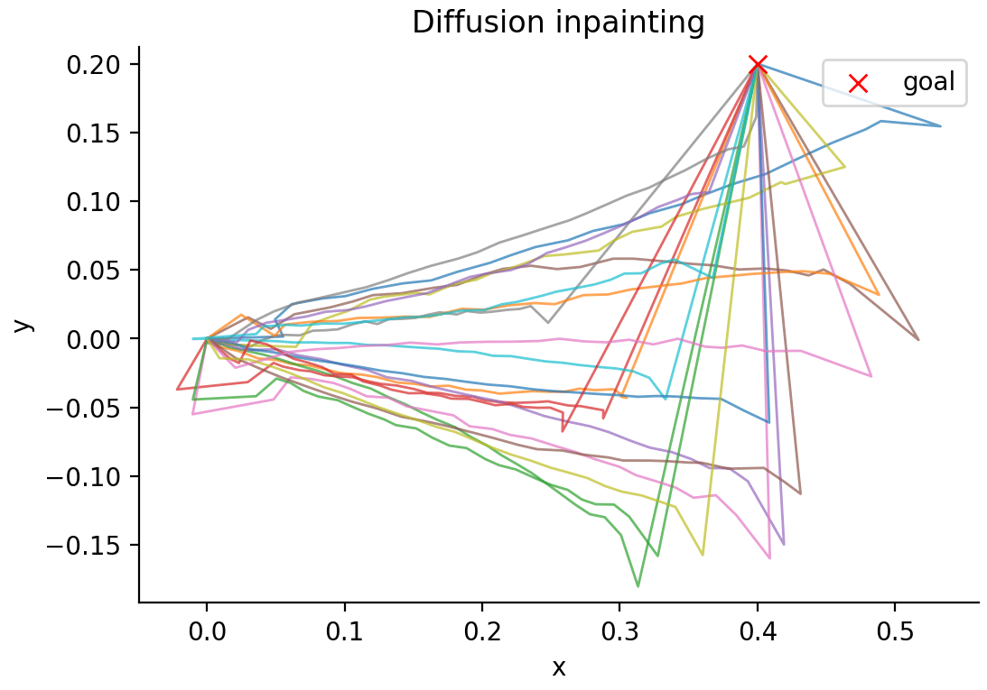
Which is not great as there are a lot of breaks in the trajectory and it looks completely out of the manifold.
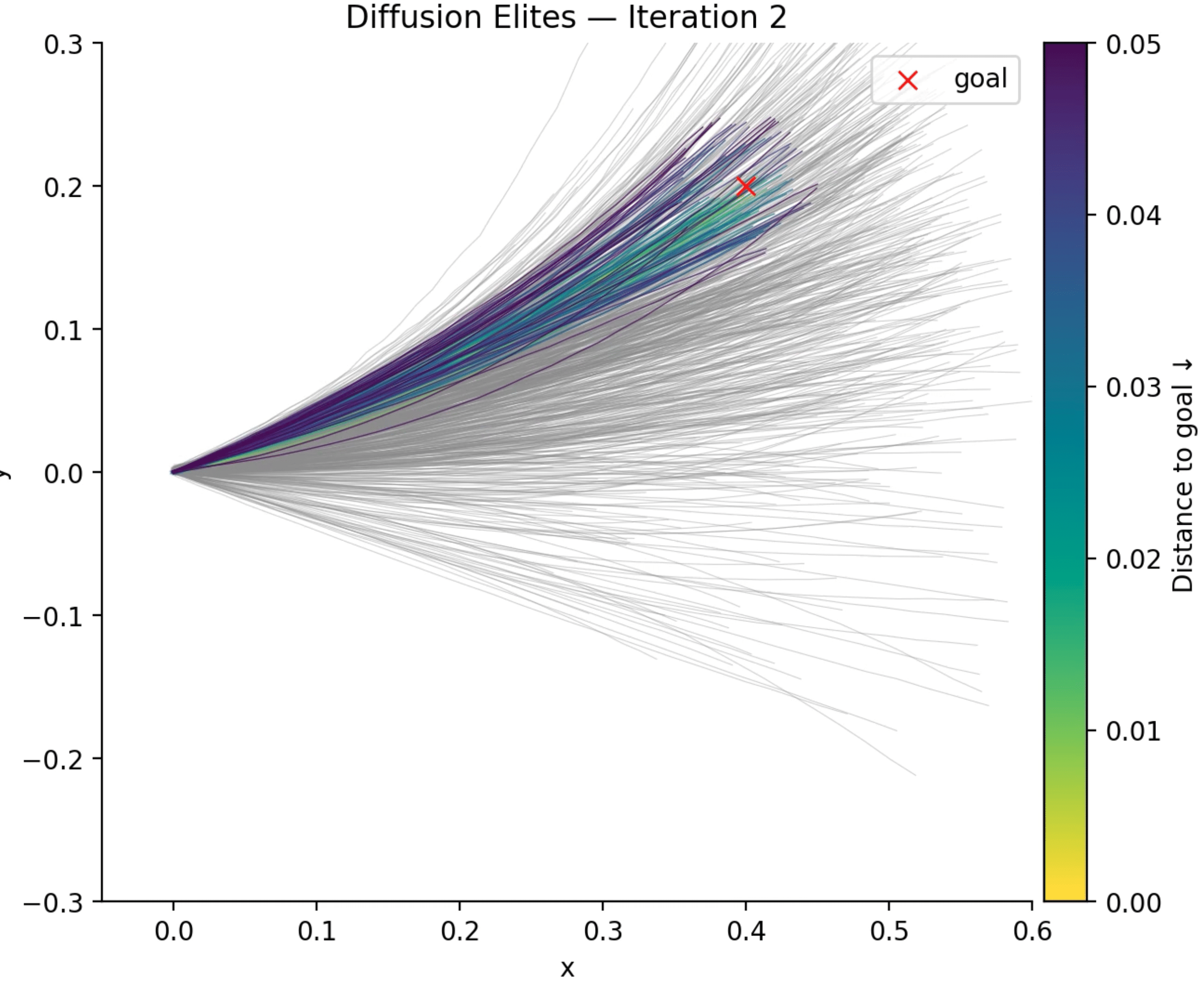
If we use Diffusion Elites though, that’s what you will see at every iteration:
In this video above, what you are seeing is the entire population in gray and the elites coloured according to their distance to the goal. There is a lot to see here, note that in the first iteration we see trajectories all over the place, which makes sense because that is what we trained it with, but note that the fraction of samples (the top-k trajectories) that we select (I’m using only 10% fraction) starts to narrow more and more to a set of solutions that are very close to the goal we wanted to reach, note how quickly it converges to it as well, in a few steps we can already see that there are a lot of solutions reaching the goal.
When you think that you can have any sort of reward (non-differentiable) to guide the search and that you can parallelize the evaluation of each sample, you will see how interesting this starts to look like. There is a lot to explore for sure and I’m planning to try on other domains as well. The nice thing about Diffusion Elites as well is that you can rely on more than a decade of convergence theory and improvements on top of the cross-entropy method and the best part is that you can implement it in a few lines of Python. I’m planning to start an open-source repository with the barebones for using it with any Diffusion model in a more structured way.
Hope you enjoyed it !
Updates
19 July 2025: added overview diagram.
– Christian S. Perone
