Hi everyone, just sharing some slides about Gemma3n architecture. I found Gemma3n a very interesting model so I decided to dig a bit further, given that information about it is still very scarce, hope you enjoy !
Download the slides PDF here.

by Christian S. Perone
Hi everyone, just sharing some slides about Gemma3n architecture. I found Gemma3n a very interesting model so I decided to dig a bit further, given that information about it is still very scarce, hope you enjoy !
Download the slides PDF here.
 It is not a secret that Diffusion models have become the workhorses of high-dimensionality generation: start with a Gaussian noise and, through a learned denoising trajectory, you get high-fidelity images, molecular graphs, or robot trajectories that look (uncannily) real. I wrote extensively about diffusion and its connection with the data manifold metric tensor recently as well, so if you are interested please take a look on it.
Now, for many engineering and practical tasks we care less about “looking real” and more about maximising a task-specific score or a reward from a simulator, a chemistry docking metric, a CLIP consistency score, human preference, etc. Even though we can use guidance or do a constrained sampling from the model, we often require differentiable functions for that. Evolution-style search methods (CEM, CMA-ES, etc), however, can shine in that regime, but naively applying them in the raw object space wastes most samples on absurd or invalid candidates and takes a lot of time to converge to a reasonable solution.
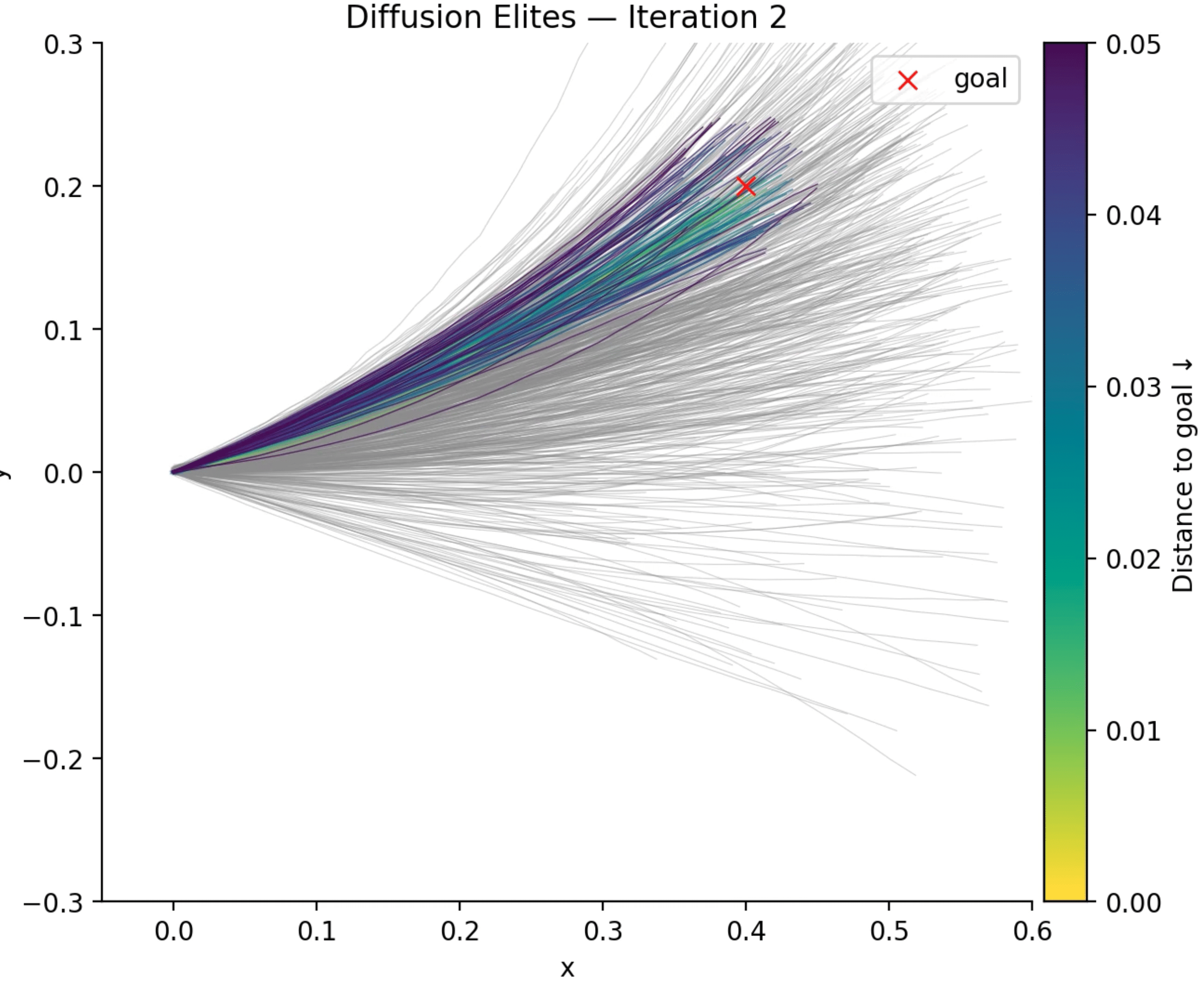
I have been experimenting on some personal projects with something that we can call “Diffusion Elites“, which aims to close this gap by letting a pre-trained diffusion model provide the prior and letting an adapted Cross-Entropy Method (CEM) steer the search inside its latent space instead. I found that this works quite well for many domains and it is also an impressively flexible method with a lot to explore (I will talk about some cases later).
To summarize, the method is as simple as the following:
This five-line loop inherits the robust, gradient-free advantages of evolutionary search while guaranteeing that every candidate lives on the diffusion model’s data manifold. In practice that means fewer wasted evaluations, faster convergence, and dramatically higher-quality solutions for many tasks (e.g. planning, design, etc). In the rest of this post I will unpack the Diffusion Elites in detail, from the algorithm to some coding examples. Diffusion Elites shows that you can explore a diffusion model and turn it into a powerful black box optimizer, it is like doing search on the data manifold itself.
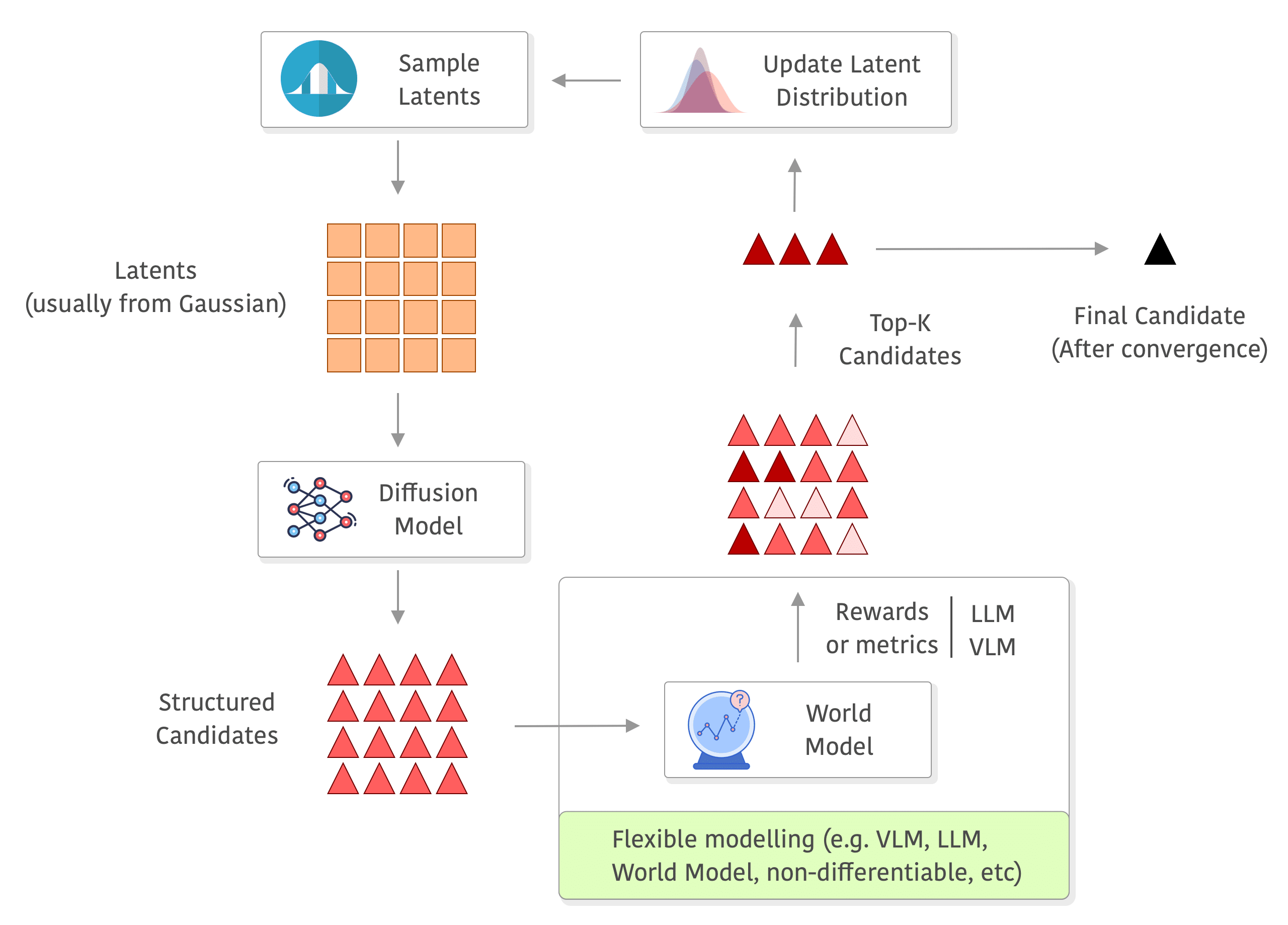
Below you can see a diagram of the process, I added a world model in the rewards to exemplify how you can use a world model and even do roll-outs there without any differentiability requirements, but you can really use anything to compute your rewards (e.g. you can also compute metrics on the outputs of the world model, or use a VLM/LLM as judge or even as world model as well):
I finally had some time over the holidays to complete the first panel of the TorchStation. The core idea is to have a monitor box that sits on your desk and tracks distributed model training. The panel shown below is a prototype for displaying GPU usage and memory. I’ll continue to post updates as I add more components. The main challenge with this board was power: the LED bars alone drew around 1.2A (when all full brightness and all lit up), so I had to use an external power supply and do a common ground with the MCU, for the panel I used a PLA Matte and 3mm. Wiring was the worst, this panel alone required at least 32 wires, but the panel will hide it quite well. I’m planning to support up to 8 GPUs per node, which aligns with the typical maximum found in many cloud instances. Here is the video, which was quite tricky to capture because of the camera metering of exposure that kept changing due to the LEDs (the video doesn’t do justice to how cool these LEDs are, they are very bright and clear even in daylight):
I’m using for the interface the Arduino Mega (which uses the ATmega2560) and Grove ports to make it easier to connect all of this, but I had to remove all VCCs from the ports to be able to supply from an external power supply, in the end it looks like this below:
                 ┌────────── PC USB (5V, ≤500 mA)
                 │
            +5 V │
                 ▼
     ┌─────────────────┐
     │  Arduino Mega   │  Data pins D2…D13, D66…D71 → LED bars
     └─────────────────┘
                ▲  GND (common reference)
                │
   ┌────────────┴──────────────┐
   │ 5V, ≥3 A switching PSU    │  ← external PSU
   └───────┬───────────┬───────┘
           │           │
           │ +5V       │ GND
           ▼           ▼
┌─────────────────────────────────┐
│ Grove Ports (VCC rail)          │ <– external 5V injected here
│ 8 × LED Bar cables              │
└─────────────────────────────────┘
PS: thanks for all the interest, here you are some discussions about VectorVFS as well:
Hacker News: discussion thread
Reddit: discussion thread
When I released EuclidesDB in 2018, which was the first modern vector database before milvus, pinecone, etc, I ended up still missing a piece of simple software for retrieval that can be local, easy to use and without requiring a daemon or any other sort of server and external indexes. After quite some time trying to figure it out what would be the best way to store embeddings in the filesystem I ended up in the design of VectorVFS.
The main goal of VectorVFS is to store the data embeddings (vectors) into the filesystem itself without requiring an external database. We don’t want to change the file contents as well and we also don’t want to create extra loose files in the filesystem. What we want is to store the embeddings on the files themselves without changing its data. How can we accomplish that ?
It turns out that all major Linux file systems (e.g. Ext4, Btrfs, ZFS, and XFS) support a feature that is called extended attributes (also known as xattr). This metadata is stored in the inode itself (ona reserved space at the end of each inode) and not in the data blocks (depending on the size). Some file systems might impose limits on the attributes, Ext4 for example requires them to be within a file system block (e.g. 4kb).
That is exactly what VectorVFS do, it embeds files (right now only images) using an encoder (Perception Encoder for the moment) and then it stores this embedding into the extended attributes of the file in the filesystem so we don’t need to create any other file for the metadata, the embedding will also be automatically linked directly to the file that was embedded and there is also no risks of this embedding being copied by mistake. It seems almost like a perfect solution for storing embeddings and retrieval that were there in many filesystems but it was never explored for that purpose before.
If you are interested, here is the documentation on how to install and use it, contributions are welcome !
* This time, this is not a technical article (but it is about philosophy of technology 😄)

This is a short opinion article to share some notes on the book by the French philosopher Gilbert Simondon called “On the Mode of Existence of Technical Objects” (Du mode d’existence des objets techniques) from 1958. Despite his significant contributions, Simondon still (and incredibly) remains relatively unknown, and it seems to me that this is partly due to the delayed translation of his works. I realized recently that his philosophy of technology aligns very well with an actionable understanding of AI/ML. His insights illuminated a lot for me on how we should approach modern technology and what cultural and societal changes are needed to view AI as an evolving entity that can be harmonised with human needs. This perspective offers an alternative to the current cultural polarization between technophilia and technophobia, which often leads to alienation and misoneism. I think that this work from 1958 provides more enlightening and actionable insights than many contemporary discussions of AI and machine learning, which often prioritise media attention over public education. Simondon’s book is very dense and it was very difficult to read (I found it more difficult than Heidegger’s work on philosophy of technology), so in my quest to simplify it, I might be guilty of simplism in some cases.

