Google’s S2, geometry on the sphere, cells and Hilbert curve
Update – 05 Dec 2017: Google just announced that it will be commited to the development of a new released version of the S2 library, amazing news, repository can be found here.
Google’s S2 library is a real treasure, not only due to its capabilities for spatial indexing but also because it is a library that was released more than 4 years ago and it didn’t get the attention it deserved. The S2 library is used by Google itself on Google Maps, MongoDB engine and also by Foursquare, but you’re not going to find any documentation or articles about the library anywhere except for a paper by Foursquare, a Google presentation and the source code comments. You’ll also struggle to find bindings for the library, the official repository has missing Swig files for the Python library and thanks to some forks we can have a partial binding for the Python language (I’m going to it use for this post). I heard that Google is actively working on the library right now and we are probably soon going to get more details about it when they release this work, but I decided to share some examples about the library and the reasons why I think that this library is so cool.
The way to the cells
You’ll see this “cell” concept all around the S2 code. The cells are an hierarchical decomposition of the sphere (the Earth on our case, but you’re not limited to it) into compact representations of regions or points. Regions can also be approximated using these same cells, that have some nice features:
- They are compact (represented by 64-bit integers)
- They have resolution for geographical features
- They are hierarchical (thay have levels, and similar levels have similar areas)
- The containment query for arbitrary regions are really fast
The S2 library starts by projecting the points/regions of the sphere into a cube, and each face of the cube has a quad-tree where the sphere point is projected into. After that, some transformation occurs (for more details on why, see the Google presentation) and the space is discretized, after that the cells are enumerated on a Hilbert Curve, and this is why this library is so nice, the Hilbert curve is a space-filling curve that converts multiple dimensions into one dimension that has an special spatial feature: it preserves the locality.
Hilbert Curve

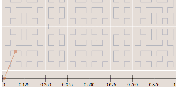
The Hilbert curve is space-filling curve, which means that its range covers the entire n-dimensional space. To understand how this works, you can imagine a long string that is arranged on the space in a special way such that the string passes through each square of the space, thus filling the entire space. To convert a 2D point along to the Hilbert curve, you just need select the point on the string where the point is located. An easy way to understand it is to use this iterative example where you can click on any point of the curve and it will show where in the string the point is located and vice-versa.
In the image below, the point in the very beggining of the Hilbert curve (the string) is located also in the very beginning along curve (the curve is represented by a long string in the bottom of the image):
Now in the image below where we have more points, it is easy to see how the Hilbert curve is preserving the spatial locality. You can note that points closer to each other in the curve (in the 1D representation, the line in the bottom) are also closer in the 2D dimensional space (in the x,y plane). However, note that the opposite isn’t quite true because you can have 2D points that are close to each other in the x,y plane that aren’t close in the Hilbert curve.
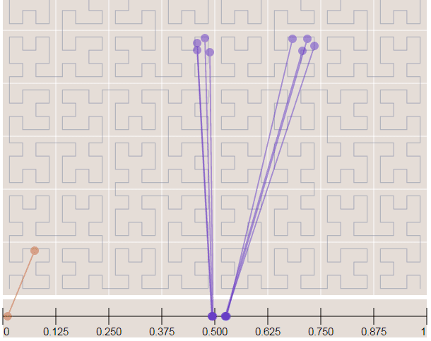
Since S2 uses the Hilbert Curve to enumerate the cells, this means that cell values close in value are also spatially close to each other. When this idea is combined with the hierarchical decomposition, you have a very fast framework for indexing and for query operations. Before we start with the pratical examples, let’s see how the cells are represented in 64-bit integers.
If you are interested in Hilbert Curves, I really recommend this article, it is very intuitive and show some properties of the curve.
The cell representation
As I already mentioned, the cells have different levels and different regions that they can cover. In the S2 library you’ll find 30 levels of hierachical decomposition. The cell level and the area range that they can cover is shown in the Google presentation in the slide that I’m reproducing below:
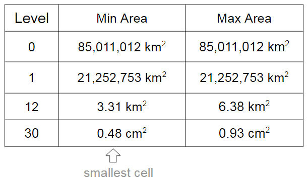
As you can see, a very cool result of the S2 geometry is that every cm² of the earth can be represented using a 64-bit integer.
The cells are represented using the following schema:
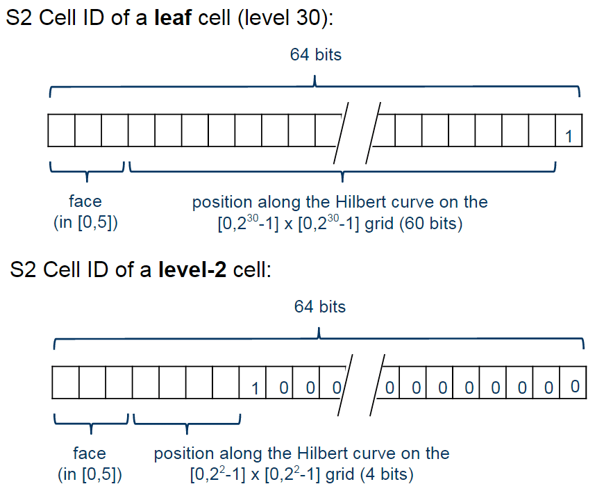
The first one is representing a leaf cell, a cell with the minimum area usually used to represent points. As you can see, the 3 initial bits are reserved to store the face of the cube where the point of the sphere was projected, then it is followed by the position of the cell in the Hilbert curve always followed by a “1” bit that is a marker that will identify the level of the cell.
So, to check the level of the cell, all that is required is to check where the last “1” bit is located in the cell representation. The checking of containment, to verify if a cell is contained in another cell, all you just have to do is to do a prefix comparison. These operations are really fast and they are possible only due to the Hilbert Curve enumeration and the hierarchical decomposition method used.
Covering regions
So, if you want to generate cells to cover a region, you can use a method of the library where you specify the maximum number of the cells, the maximum cell level and the minimum cell level to be used and an algorithm will then approximate this region using the specified parameters. In the example below, I’m using the S2 library to extract some Machine Learning binary features using level 15 cells:
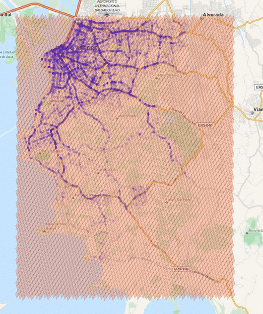
The cells regions are here represented in the image above using transparent polygons over the entire region of interest of my city. Since I used the level 15 both for minimum and maximum level, the cells are all covering similar region areas. If I change the minimum level to 8 (thus allowing the possibility of using larger cells), the algorithm will approximate the region in a way that it will provide the smaller number of cells and also trying to keep the approximation precise like in the example below:
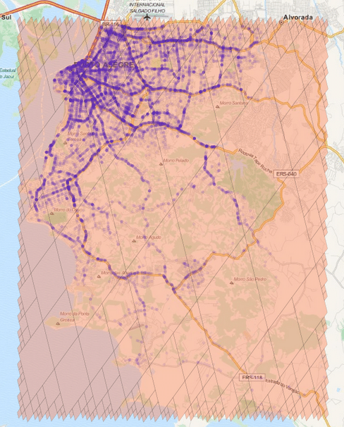
As you can see, we have now a covering using larger cells in the center and to cope with the borders we have an approximation using smaller cells (also note the quad-trees).
Examples
* In this tutorial I used the Python 2.7 bindings from the following repository. The instructions to compile and install it are present in the readme of the repository so I won’t repeat it here.
The first step to convert Latitude/Longitude points to the cell representation are shown below:
>>> import s2
>>> latlng = s2.S2LatLng.FromDegrees(-30.043800, -51.140220)
>>> cell = s2.S2CellId.FromLatLng(latlng)
>>> cell.level()
30
>>> cell.id()
10743750136202470315
>>> cell.ToToken()
951977d377e723ab
As you can see, we first create an object of the class S2LatLng to represent the lat/lng point and then we feed it into the S2CellId class to build the cell representation. After that, we can get the level and id of the class. There is also a method called ToToken that converts the integer representation to a compact alphanumerical representation that you can parse it later using FromToken method.
You can also get the parent cell of that cell (one level above it) and use containment methods to check if a cell is contained by another cell:
>>> parent = cell.parent()
>>> print parent.level()
29
>>> parent.id()
10743750136202470316
>>> parent.ToToken()
951977d377e723ac
>>> cell.contains(parent)
False
>>> parent.contains(cell)
True
As you can see, the level of the parent is one above the children cell (in our case, a leaf cell). The ids are also very similar except for the level of the cell and the containment checking is really fast (it is only checking the range of the children cells of the parent cell).
These cells can be stored on a database and they will perform quite well on a BTree index. In order to create a collection of cells that will cover a region, you can use the S2RegionCoverer class like in the example below:
>>> region_rect = S2LatLngRect(
        S2LatLng.FromDegrees(-51.264871, -30.241701),
        S2LatLng.FromDegrees(-51.04618, -30.000003))
>>> coverer = S2RegionCoverer()
>>> coverer.set_min_level(8)
>>> coverer.set_max_level(15)
>>> coverer.set_max_cells(500)
>>> covering = coverer.GetCovering(region_rect)
First of all, we defined a S2LatLngRect which is a rectangle delimiting the region that we want to cover. There are also other classes that you can use (to build polygons for instance), the S2RegionCoverer works with classes that uses the S2Region class as base class. After defining the rectangle, we instantiate the S2RegionCoverer and then set the aforementioned min/max levels and the max number of the cells that we want the approximation to generate.
If you wish to plot the covering, you can use Cartopy, Shapely and matplotlib, like in the example below:
import matplotlib.pyplot as plt

from s2 import *

from shapely.geometry import Polygon

import cartopy.crs as ccrs
import cartopy.io.img_tiles as cimgt

proj = cimgt.MapQuestOSM()
plt.figure(figsize=(20,20), dpi=200)
ax = plt.axes(projection=proj.crs)

ax.add_image(proj, 12)
ax.set_extent([-51.411886, -50.922470,
               -30.301314, -29.94364])

region_rect = S2LatLngRect(
    S2LatLng.FromDegrees(-51.264871, -30.241701),
    S2LatLng.FromDegrees(-51.04618, -30.000003))

coverer = S2RegionCoverer()
coverer.set_min_level(8)
coverer.set_max_level(15)
coverer.set_max_cells(500)
covering = coverer.GetCovering(region_rect)

geoms = []
for cellid in covering:
    new_cell = S2Cell(cellid)
    vertices = []
    for i in xrange(0, 4):
        vertex = new_cell.GetVertex(i)
        latlng = S2LatLng(vertex)
        vertices.append((latlng.lat().degrees(),
                         latlng.lng().degrees()))

    geo = Polygon(vertices)
    geoms.append(geo)

print "Total Geometries: {}".format(len(geoms))

ax.add_geometries(geoms, ccrs.PlateCarree(), facecolor='coral',
                  edgecolor='black', alpha=0.4)
plt.show()
And the result will be the one below:
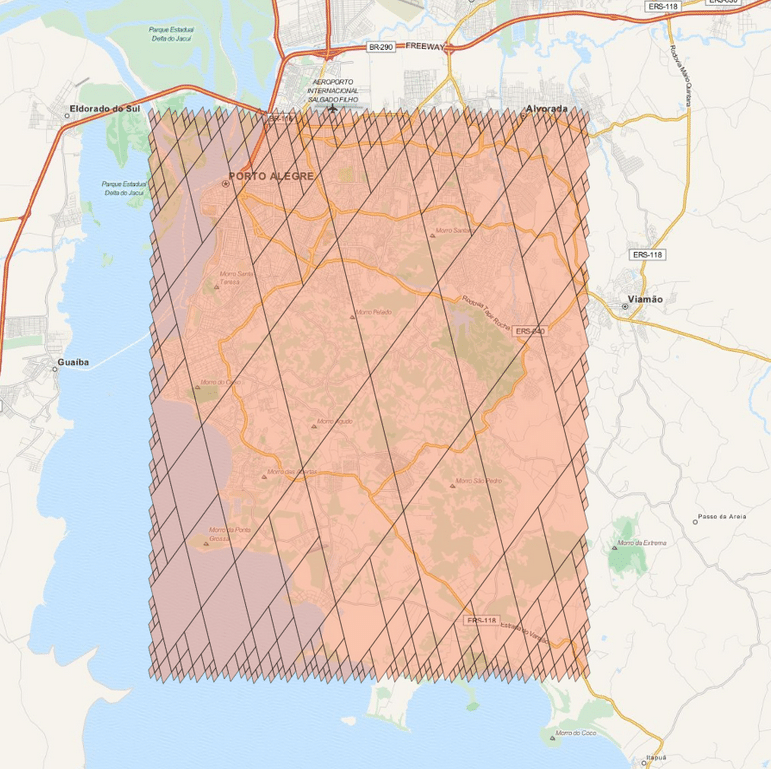
There are a lot of stuff in the S2 API, and I really recommend you to explore and read the source-code, it is really helpful. The S2 cells can be used for indexing and in key-value databases, it can be used on B Trees with really good efficiency and also even for Machine Learning purposes (which is my case), anyway, it is a very useful tool that you should keep in your toolbox. I hope you enjoyed this little tutorial !
– Christian S. Perone

Great post! Thank you for digging this up and articulating it so well. Definitely sharing this one around the office. Cheers!
Thanks John, I’m really glad you liked it.
Interesting, useful and straightforward to follow. Thanks.
I created a pure Python implementation here as well https://github.com/qedus/sphere
This is very nice, thanks for the effort !
this is just a quad tree right?
+1
It’s a quadtree projected onto the unit sphere, plus using the Hilbert curve for a fast mapping between integer indices and cells.
Thank you for a great article.
I wonder whether we can apply the above methodology in order to analyze posts from the social media streams. Ideas are welcomed!
Best.
Iason
@iason
http://www.postmechanics.com
Thanks for this post. Helped me quite a lot. You had posted this link on my question in stack exchange.
I have run the same examples of getting cellIDs in Java. It works well. However, I have some question which you might be able to answer or give direction for the same:
1) How is cell ID different from geo-hash? Or is it same?
2) Can routing be done with S2?
3) I came across S2 library when I was trying to do ETA(time of arrival) analysis with vehicle/bike data I had. I read that Google, foursquare, Uber use this library. I had posted the same question : gis. stackexchange. com /questions/152719/postgis-for-gpx-analysis. few days back. Can you make out any approach to solve the same?
Hi, I would say that S2 is a kind of a geohash with different properties. Routing cannot be done with S2, S2 isn’t a algorithm for routing but for geometry on sphere, it can be used to generate a covering for a route but not for routing itself, for that I suggest you to look at the traditional routing algorithms like A-star, etc.
Your problem is a wide open problem, you can use Machine Learning methods to approximate the time it will take to go to a certain destination at certain time of the day using historical records, there are a lot of methods you can use, but I don’t really know any benchmark (of results performance) between different models for that, try searching for papers about that, you should certainly find something related with your problem.
Thats great what you said – “it can be used to generate a covering for a route but not for routing itself,”
It means, if I have a set of points along a route, I can create a covering with S2 cells.
I have to pre-calculate from historical data, what time it takes for the cells to move at a particular time of the day. I can sum them up and create the ETA.
But, what is best use of Hilbert curve here? I am still confused w.r.t usecases of the same. Can S2 cells be enriched with more information, like in my case with time? And Hilbert curve might give me faster lookup of this information?
Not sure if the questions are still on your mind, but if they are :
GeoHash and S2Cells are made for the same purpose of dividing a spherical geospatial plane into partitions / cells while preserving locality (meaning 2 geospatially adjacent cells should have a “similar” hash code / cell id)
GeoHash does that by taking the sphere and dividing it to 2 parts, one is coded 1 the other is 0 (lvl1), taking one of the parts and continuing the same process will result in a new lvl with finer granularity and longer GeoHash Code.
This method as you see is linear in embedding (lon,lat -> geohash code) which makes it super fast but lacks accuracy (mostly near equator lines) and therefore has large variance on cell sized (2 adjacent cells can vary largely in cell area)
S2Cell embedding is more complex, bounding the sphere with a cube, dividing each cube face to 4 parts with a quad-tree (and each part to smaller parts, therefrom comes the notion of s2 cell levels which are the level in the tree) and finally enumerating tree leaves to s2cell IDs (long codes) using a hilbert space filling curve.
Embedding is therefore quadratic (quad-tree) which is a bit slower then geohash but taking into account projection from a sphere to a cube which trades off with less variance regarding to cell area (adjacent cells are closer in size, so you get less errors when aggregating appearances in every cell and comparing them to one another – is this a “hotspot”?)
Hope this helps!
S2 Cells are awesome, and this was a great piece!
(all the data provided here is “public” meaning you could with some great effort deduce it from the presentation above and the source code :))
One more resource that might help is this presentation :
http://www.slideshare.net/DanielMarcous/geo-data-analytics
Regards,
Daniel Marcous.
“However, note that the opposite isn’t quite true because you can have 2D points that are close to each other in the x,y plane that aren’t close in the Hilbert curve.”
I noticed this and wonder what the implications are. It seems that it would make some of the operations “asymmetric”. Is this a problem in practice?
Great article. Many thanks!
“you’re not going to find any documentation or articles about the library anywhere except for a paper by Foursquare , a Google presentation and the source code comments.”.
Hi! Where can i find the paper from Foursquare? I’v got confuse in the class S2CellId in the java version, how dose it generate a lookup table recursively, It’s too much bit operations makes the code hard to read.
Hi Christian,
Really informative post.
Were you able to create a regionCoverer using polygons? Do you have any example to do the same?
Hi Christian — I think the library from the micolous repository is mapping coordinates to the wrong cube face, causing the more diamond-like cell shapes. I did a cover using some coordinates in Washington DC. The micolous library put them on face 101 while s2map put them on 100. I posted a comparison slide here: http://imgur.com/ymvw3o2
Christian, this is a great article. I have a question- Does the S2 cell lie on the idealized sphere, or does it mirror the contour of the actual surface? Also since it assumes a sphere, is there an issue because the actual shape of the earth is an oblate ellipsoid?
This is Fantastic. Thanks Christian and I am sorry for not able to find a word other than fantastic which really could compliment you sufficiently for this.
Hi Christian,
Thank you so much for this much helpful tutorial.
So looking at this data about the area range of cells for different levels (http://blog.christianperone.com/wp-content/uploads/2015/08/s2_cell_area.png), it shows the ranges for levels 0,1,12,30. How can I get the ranges of the other cells?
Thanks
Could you find ranges for other cells?
Can S2 be used to make geo-radial query? For example, say, I have a set of lat/long, and I want to find out which among those are with in a given distance from a given location. Basically combination of GeoAdd and GeoRadis Redis commands.
Really awesome post! The better summary that I’ve found on my study about GeoQuery and GeoIndex methods.
Thanks a lot for that and for awesome Pingbacks!
Great post.
If you had a load of lat/long data in a database – how would you go about creating s2 functions to go from lat/long to a cell_id at a given level.
I have lat/long data in google bigquery and am wondering if i could use UDF’s to get s2 functionality in BQ to avoid having to send the data back out to python or somewhere else for processing.
Cheers
Andy
This is a great illustration of how the S2Cell hierarchy works. Thanks very much.
Great post, updates for Python 3.5 and s2sphere (python)
import s2sphere as s2import matplotlib.pyplot as plt
from shapely.geometry import Polygon
import cartopy.crs as ccrs
import cartopy.io.img_tiles as cimgt
proj = cimgt.OSM()
plt.figure(figsize=(20, 20), dpi=200)
ax = plt.axes(projection=proj.crs)
ax.add_image(proj, 12)
ax.set_extent([-51.411886, -50.922470,
-30.301314, -29.94364])
region_rect = s2.LatLngRect(
s2.LatLng.from_degrees(-51.264871, -30.241701),
s2.LatLng.from_degrees(-51.04618, -30.000003))
coverer = s2.RegionCoverer()
coverer.min_level=8
coverer.max_level=15
coverer.max_cells=500
covering = coverer.get_covering(region_rect)
geoms = []
for cellid in covering:
new_cell = s2.Cell(cellid)
vertices = []
for i in range(0, 4):
vertex = new_cell.get_vertex(i)
latlng = s2.LatLng.from_point(vertex)
vertices.append((latlng.lat().degrees,latlng.lng().degrees))
geo = Polygon(vertices)
geoms.append(geo)
print("Total Geometries: {}".format(len(geoms)))
ax.add_geometries(geoms, ccrs.PlateCarree(), facecolor='coral', edgecolor='black', alpha=0.4)
plt.show()
Hi Al ! Great thanks for the contribution !
Hi Christian,
Thanks so much for this blog post !
As there is no documentation for the S2Polygon object, I wonder what arguments it needs to be fed.
Could you give me a pointer ?
Thank you !
Whether or not sharing your experience, breaking news, or
no matter’s in your thoughts, you’re in good firm on Blogger.
Everything posted made a bunch of sense. However, consider this, suppose you were to write a awesome title?
I am not suggesting your information isn’t good, but what if you added a title that grabbed folk’s attention? I mean Google’
s S2, geometry on the sphere, cells and Hilbert curve | Terra Incognita is a little vanilla.
You could look at Yahoo’s home page and note how they create news
headlines to get people to click. You might add a video or a related picture or
two to get people interested about what you’ve got to say.
Just my opinion, it would bring your website a little livelier.
Excelente Post! Thanks Chris!
Chris….I don’t know why it took me so long to find this wonderful post, but it has been a tremendous benefit to me!!!
Thank you very much!
Thanks for the feedback Ryan !!!
Thanks Christian S. Perone for this article. It has helped to pursued to use the S2 Google library to do our geo spatial queries for a fleet tracking system we are developing. Those who are interested in a very cool node.js implementation please look at Andrea’s typescript implementation of the Google S2 which plays nicely in node on github (nodes2ts). https://github.com/vekexasia/nodes2-ts
Thanks for the feedback, I’m really glad you liked and that it was useful for you.
Excellent way of telling, and pleasant article to take facts about my presentation topic, which i
am going to deliver in college.
Thank you for the auspicious writeup. It in truth used to be a enjoyment account it.
Glance complicated to more delivered agreeable from you! By the
way, how can we be in contact?
Thanks a lot for this amazing tutorial Christian!
I have a lot of doubts though. Would be great if you can help. 🙂
In the example, you have created a rect region from two points. How does that work?
I want to create a region from a thousand points(latlong). And then divide it region in the cells. How can I do that?
I can see there is a method addPoint for rect in c++ library, but nothing in python.
Can you help? Thanks a lot!
Hi Christian,
Many thanks for the article, really comprehensive! My only question would be how the appropriate face (out of the 6 faces of the cube) is decided to project a given (lat,lng) region on.
Best,
– ZP
Edit:
My original impression was that each region (or point is potentially projected linearly on more than one cube faces (the ones where it is “visible from). However, it seems that each region (or point) has a unique projection onto the cube, as the projection of the line segment starting from the Earth center, passing through the region (or point) and ending at a point in one of the six cube faces (as shown in Google’s presentation: https://docs.google.com/presentation/d/1Hl4KapfAENAOf4gv-pSngKwvS_jwNVHRPZTTDzXXn6Q/view#slide=id.i15).
A new update is out now with a lot more docs as well:
https://opensource.googleblog.com/2017/12/announcing-s2-library-geometry-on-sphere.html
Amazing, thanks for letting me know !
Nice post Christian.
How do I use this library with android studio?
It’s very effortles to find out any matter on web as compared to textbooks, as I found this post aat this web page.
Hi Christian,
Thanks a lot for this amazing blog. It is just awesome.
I have one use case where I have geo location of users and a point in the city and I need to find users who are within 5kms radius of that point. I could represent locations of user and the point with S2 cell id. But how would I query that?
Do I need to load data for all the users inmemory to my application and then use library to find my target users. Or can I store data for all the users in a database and make query on S2 cell ids as S2 cell id is using Hilbert curve so we know that geo points who have closer S2 cell ids are closer in distance with each other.
Or is there any other method which I am missing
Thanks for the help in advance
Hi,
Saw this blog very late. I am also waiting for reply to the question you posted. By any chance did you solve the problem.
Hi Aman,
I posted your question in other way at StackOverFlow.
Luckily, some one had answered. Here is the Link
https://stackoverflow.com/questions/57686995/how-to-perform-the-search-operation-using-google-s2-geometry
Were you able to install this using python3 – https://github.com/google/s2geometry/issues/46 ?
Hi Christian, thanks for this article. I just wanted to mention that I had to use `OSM` instead of `MapQuestOSM ` and switch the order of lat and lng when appending to `geoms`
So instead of:
“`
vertices.append((latlng.lat().degrees(),
latlng.lng().degrees()))
“`
I did:
“`
vertices.append((latlng.lng().degrees(),
latlng.lat().degrees()))
“`
Everything composed wass very logical. However, what about this?
what if you added a little information? I ain’t suggesting your information is not good, but
suppose you added a post title that grabbed folk’s attention?
I mean Google's S2, geometry on thhe sphere, cells and Hilbert cuurve | Terra Incognita is kinda plain. You could glance at Yahoo’s front page
and see how they create news headlines to get
people interested. You mignt add a video orr a related
picture or two to get readers interested about what you’ve got
to say. In my opinion, it would make your blog a little bit more interesting.
Hello. I see that you don’t update your site too often. I know that writing articles is time consuming and boring.
But did you know that there is a tool that allows you to create
new articles using existing content (from article directories or other websites from your niche)?
And it does it very well. The new articles are unique and pass the copyscape test.
You should try miftolo’s tools
To some individuals, junk food appears inevitable even though they are aware of the inevitable risk fast food
diet regimens could possibly trigger.
Everything is very open with a precise description of the challenges.
It was really informative. Your site is useful. Many thanks for sharing!
Anyone got a javascript version? I’m just a reg guy with a reg map that I’d like to implement this to.
Pokemon go brought me here, the amazing post made me stay!
Magnificent goods from you, man. I’ve understand your stuff previous to
and you are just too great. I actually like what you have acquired here, really like what you
are stating and the way in which you say it. You make it entertaining and you still care for to keep it wise.
I can not wait to read far more from you. This
is really a tremendous site.
Has anybody actually got this working with Python 3 – https://github.com/google/s2geometry/issues/46 ?
I have been exploring for a bit for any high-quality articles or weblog posts in this sort of house .
Exploring in Yahoo I ultimately stumbled upon this web site.
Reading this info So i am happy to show that I’ve a very excellent uncanny feeling I came upon just what
I needed. I most indisputably will make certain to don?t omit this website and give
it a look regularly.
Helpful information. Fortunate me I found your site by chance, and I am stunned why this accident didn’t took
place earlier! I bookmarked it.
Thanks Christian, this is a very helpful post!
I am actually thankful to the holder of this site
who has shared this great article at at this time.
Christian,
Thanks for pulling this all together, it’s super useful 😀
Note that, you need to be wary of the order that lats/lons are provided to each of the packages i.e.,
– s2 takes (lat, lon) order
– shapely takes (x, y) or (lon, lat) order
– cartopy’s set_extent takes (x0, x1, y0, y1) or (lon0, lon1, lat0, lat1) order
Your example code seems to follow this, but in lines 35-36 you’ve given s2 (lat, lon) order to specify each geometry vertex to a shapely Polygon, which should be in (lon, lat) order instead.
Also, I’m keen to expose the whole s2geometry API to Python, rather than be limited to the restricted API coverage provided by the google/s2geometry SWIG Python bindings.
Inspired by you blog, I’ve started that journey at https://github.com/bjlittle/docker-s2geometry