From Modis Rapid Response System site:

The MODIS Rapid Response System was developed to provide daily satellite images of the Earth’s landmasses in near real time. True-color, photo-like imagery and false-color imagery are available within a few hours of being collected, making the system a valuable resource (…).
The Moderate Resolution Imaging Spectroradiometer (MODIS) flies onboard NASA’s Aqua and Terra satellites as part of the NASA-centered international Earth Observing System. Both satellites orbit the Earth from pole to pole, seeing most of the globe every day. Onboard Terra, MODIS sees the Earth during the morning, while Aqua MODIS orbits the Earth in the afternoon.

One thing that a few people know is that everyone can have access to a near real-time moderate resolution images from two NASA satellites (Aqua and Terra) which orbits the earth from pole to pole every day and captures images and data like thermal anomalies from the most part of the globe.

In this post, I’ll show how to get and plot those imagery and data to a map using Python and Matplotlib + Basemap toolkit.

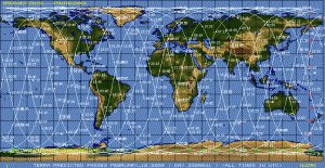
The Aqua and Terra orbits

What do the orbit track maps show?

The response is from NASA site,

The maps have a series of white lines with tick marks on them that show what time (using Coordinated Universal Time, or UTC) the satellite will be passing over a particular location on Earth on a given day. The white lines represent the center of the swath. The time stamps mark the start of the northern (Terra) or southern (Aqua) edge of each 5-minute data collection period. An image acquired at that location will span roughly 1150 kilometers on either side of the tick mark. Every day there are two passes over most areas: one daylight pass, and one nighttime pass. At this point the MODIS Rapid Response System produces images for the daylight passes only.

The image products

The MODIS also provides different band combined images, like the Band 3-6-7 combination, which helps distinguish the liquid water from frozen water. You can find more information about the other band combinations on the FAQ.

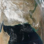
Well, the real-time imagery is available here, those images are Level-2 images, which means that they are not yet corrected, you will see that they appears with some distortion:

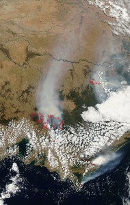
But we have some subsets available here, and they are automatically generated in near-real-time for various applications users. Here is an example of recent fire in Australia (the red markers are the thermal anomalies, click in the image to enlarge):

In the image we can see the smoke caused by the fires. This photo is from 09 Feb. 2009, 04:40 UTC, taken by the Aqua satellite.

The active fire hotspots data

There are some information that will be helpful for us too, is the hotspot/fire products, those products are from FIRMS –  Fire Information for Resource Management System -, the objective of FIRMS is:

FIRMS provides MODIS hotspot / fire products to natural resource managers around the world in easy to use formats.

The active fire/hotspots are available on txt and in shape files format, to use the txt, you must ask for a permission, but the shape files is public available at the firedata section of the site. We will use the Global firedata, which is available in the lasts 24 hrs, 48 hrs or 7 days.

The shape files are updated every 4 hours and uses the WGS84 projection, if you are interested about the shape files, read the FAQ on the site.

The code

[See the full source-code]

Now that we have the imagery and the shape data files with the active fire hotspots, let’s begin to code:

1) Downloading the MODIS image and metadata

To download the image from MODIS, we use the available zip file with the image and some metadata files, it is available in this URL:

http://rapidfire.sci.gsfc.nasa.gov/subsets/?subset=[Subset name].[Year][Day of the year].[Satellite].[Pixel size].zip

An example of this URL is:

http://rapidfire.sci.gsfc.nasa.gov/subsets/?subset=FAS_Brazil5.2009041.terra.2km.zip

This URL will download the subset package of the subset “FAS_Brazil5” of 041/2009 taken by the “Terra” satellite and with a pixel size of 2KM.

To download this file, we will use a defined function that will download it using the urllib2 Python module, see the full source code to view all the functions, I will omit some of them for the sake of brevity.

This piece of code will download the zip file in the data.zip and decompress it on a temporary folder:

   download(URL_RAPIDFIRE_SUBSET, "data.zip")
   zipf    = zipfile.ZipFile('data.zip')
   tempdir = tempfile.mkdtemp() 

   for name in zipf.namelist():
      data    = zipf.read(name)
      outfile = os.path.join(tempdir, name)
      f       = open(outfile, 'wb')
      f.write(data)
      f.close() 

   zipf.close()

The next step is to download the image metadata, this metadata file contains the follow:

subset: FAS_Brazil5
date: 2009041 (02/10/09)
satellite: Terra
projection: Plate Carree
projection center lon: 0.0000
projection center lat: 0.0000
UL lon: -57.2947
UL lat: -25.3305
UR lon: -48.2029
UR lat: -25.3305
LR lon: -48.2029
LR lat: -35.6727
LL lon: -57.2947
LL lat: -35.6727

This information will be used to set the Matplotlib Basemap parameters of the upper left corner latitude, etc.

Here is the code that will download and parse the metadata file:

   metadata = downloadString(URL_METADATA)
   ll_lon = parseTerm(metadata, "LL lon")
   ll_lat = parseTerm(metadata, "LL lat")
   ur_lon = parseTerm(metadata, "UR lon")
   ur_lat = parseTerm(metadata, "UR lat")

2) Downloading and parsing the active fire hotspots data – shape file

The next step is to download and parse the shape file that have the active fire hotspots data, this piece of code will download the zipped shape file:

   download(URL_FIRE_SHAPES, "shapes.zip")
   zipf = zipfile.ZipFile('shapes.zip') 

   for name in zipf.namelist():
      data    = zipf.read(name)
      outfile = os.path.join(tempdir, name)
      f       = open(outfile, 'wb')
      f.write(data)
      f.close()
   zipf.close()

And this is the source code to parse the shape file using the dbflib (included in the Basemap toolkit of Matplotlib):

   shape_path = os.path.join(tempdir, 'Global_%s' % FIRE_LASTS)
   dbf        = dbflib.open(shape_path)
   rec_count  = dbf.record_count()

   xlist      = [dbf.read_record(i)['LONGITUDE'] for i in xrange(rec_count)]
   ylist      = [dbf.read_record(i)['LATITUDE'] for i in xrange(rec_count)]
   confidence = [dbf.read_record(i)['CONFIDENCE'] for i in xrange(rec_count)]
   dbf.close()

This routine will create 3 lists used to plot the fire hotspots on the map, the first list is the Longitude, the second is the Latitude, this two lists gives our x/y coord. on the map, and the “confidence” list, the confidence represents the quality of individual hotspots/fire pixels, as the FIRMS FAQ says:

A detection confidence intended to help users gauge the quality of individual hotspot/fire pixels is included in the Level 2 fire product. This confidence estimate, which ranges between 0% and 100%, is used to assign one of the three fire classes (low-confidence fire, nominal-confidence fire, or high-confidence fire) to all fire pixels within the fire mask. In the Collection 4 fire product this confidence estimate does not adequately identify highly questionable, low confidence fire pixels. Such pixels, which by design should have a confidence close to 0%, are too often assigned much higher confidence estimates of 50% or higher. This will be corrected for Collection 5.

3) Plotting the map with matplotlib

Now, we have all the information to plot the map, we have the last true-color image taken by the satellite, and we have the fire hotspot data of the lasts 24 hrs, the next step is to create a map and plot those information, this is the code used to do that:

   m = Basemap(projection='cyl', llcrnrlat=ll_lat, urcrnrlat=ur_lat,\
               llcrnrlon=ll_lon, urcrnrlon=ur_lon, resolution='h')
   m.drawcoastlines()
   m.drawmapboundary(fill_color='aqua')
   m.scatter(xlist, ylist, 20, c=confidence, cmap=p.cm.hot, marker='o', edgecolors='none', zorder=10)
   m.imshow(image_modis)

The final plot result

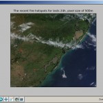
This is the final plot result, the color dots on the map is the active fire/hotspots for the lasts 24 hrs, the color is relative with the confidence value, which is from 1 to 100, this value is normalized the Matplotlib and then it is show using a color map, I’m using the “hot” colormap.

This is a plot from the south of Brazil, the image is 500m pixel size, from Terra satellite, taken in 10 Feb 2009 using the subset FAS_Brazil5.

[See the full source code]

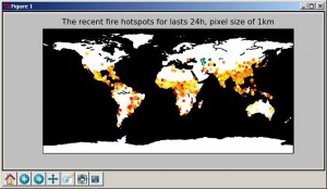
You can change the script and just plot the global shape file, the result will look like this:

This is a fire hotspot global plot of the lasts 24 hrs, data from 11 Feb. 2009.

Images courtesy of MODIS Rapid Response Project at NASA/GSFC

More information

Fire Information for Resource Management System

MODIS Rapid Response System

GLCF – Global Land Cover Facility