Read the first part of this tutorial: Text feature extraction (tf-idf) – Part I.
This post is a continuation of the first part where we started to learn the theory and practice about text feature extraction and vector space model representation. I really recommend you to read the first part of the post series in order to follow this second post.
Since a lot of people liked the first part of this tutorial, this second part is a little longer than the first.
Introduction
In the first post, we learned how to use the term-frequency to represent textual information in the vector space. However, the main problem with the term-frequency approach is that it scales up frequent terms and scales down rare terms which are empirically more informative than the high frequency terms. The basic intuition is that a term that occurs frequently in many documents is not a good discriminator, and really makes sense (at least in many experimental tests); the important question here is: why would you, in a classification problem for instance, emphasize a term which is almost present in the entire corpus of your documents ?
The tf-idf weight comes to solve this problem. What tf-idf gives is how important is a word to a document in a collection, and that’s why tf-idf incorporates local and global parameters, because it takes in consideration not only the isolated term but also the term within the document collection. What tf-idf then does to solve that problem, is to scale down the frequent terms while scaling up the rare terms; a term that occurs 10 times more than another isn’t 10 times more important than it, that’s why tf-idf uses the logarithmic scale to do that.
But let’s go back to our definition of the ")


To overcome this problem, the term frequency
Vector normalization
Suppose we are going to normalize the term-frequency vector 

d4: We can see the shining sun, the bright sun.
And the vector space representation using the non-normalized term-frequency of that document was:
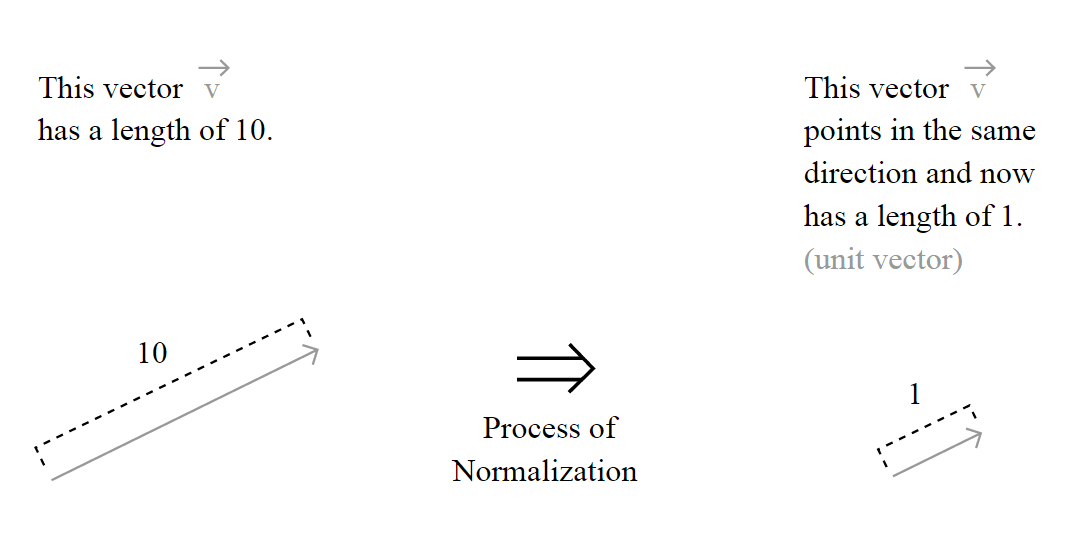
To normalize the vector, is the same as calculating the Unit Vector of the vector, and they are denoted using the “hat” notation: 


Where the 

The unit vector is actually nothing more than a normalized version of the vector, is a vector which the length is 1.
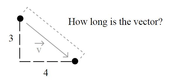
But the important question here is how the length of the vector is calculated and to understand this, you must understand the motivation of the
Lebesgue spaces
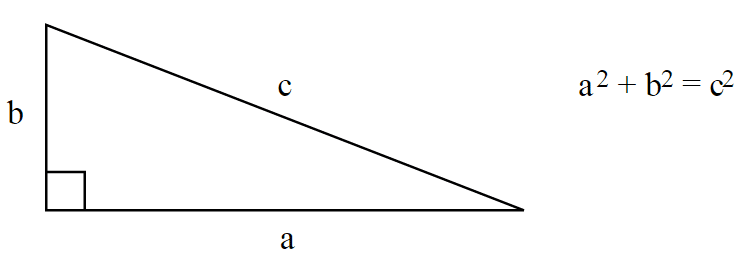
Usually, the length of a vector ")

But this isn’t the only way to define length, and that’s why you see (sometimes) a number 

^\frac{1}{p}")
and simplified as:
^\frac{1}{p}")
So when you read about a L2-norm, you’re reading about the Euclidean norm, a norm with 
When you read about a L1-norm, you’re reading about the norm with 
")
Which is nothing more than a simple sum of the components of the vector, also known as Taxicab distance, also called Manhattan distance.

Taxicab geometry versus Euclidean distance: In taxicab geometry all three pictured lines have the same length (12) for the same route. In Euclidean geometry, the green line has length 
Source: Wikipedia :: Taxicab Geometry
Note that you can also use any norm to normalize the vector, but we’re going to use the most common norm, the L2-Norm, which is also the default in the 0.9 release of the scikits.learn. You can also find papers comparing the performance of the two approaches among other methods to normalize the document vector, actually you can use any other method, but you have to be concise, once you’ve used a norm, you have to use it for the whole process directly involving the norm (a unit vector that used a L1-norm isn’t going to have the length 1 if you’re going to take its L2-norm later).
Back to vector normalization
Now that you know what the vector normalization process is, we can try a concrete example, the process of using the L2-norm (we’ll use the right terms now) to normalize our vector ")

}{\sqrt{0^2 + 2^2 + 1^2 + 0^2}} \\ \\ \hat{v_{d_4}} = \frac{(0,2,1,0)}{\sqrt{5}} \\ \\ \small \hat{v_{d_4}} = (0.0, 0.89442719, 0.4472136, 0.0)")
And that is it ! Our normalized vector 
Note that here we have normalized our term frequency document vector, but later we’re going to do that after the calculation of the tf-idf.
The term frequency – inverse document frequency (tf-idf) weight
Now you have understood how the vector normalization works in theory and practice, let’s continue our tutorial. Suppose you have the following documents in your collection (taken from the first part of tutorial):
Train Document Set:

d1: The sky is blue.
d2: The sun is bright.

Test Document Set:

d3: The sun in the sky is bright.
d4: We can see the shining sun, the bright sun.
Your document space can be defined then as 


Let’s see now, how idf (inverse document frequency) is then defined:
 = \log{\frac{\left|D\right|}{1+\left|\{d : t \in d\}\right|}}")
where 
 \neq 0")
The formula for the tf-idf is then:
 = \mathrm{tf}(t, d) \times \mathrm{idf}(t)")
and this formula has an important consequence: a high weight of the tf-idf calculation is reached when you have a high term frequency (tf) in the given document (local parameter) and a low document frequency of the term in the whole collection (global parameter).
Now let’s calculate the idf for each feature present in the feature matrix with the term frequency we have calculated in the first tutorial:

Since we have 4 features, we have to calculate ")
")
")
")
 = \log{\frac{\left|D\right|}{1+\left|\{d : t_1 \in d\}\right|}} = \log{\frac{2}{1}} = 0.69314718")
 = \log{\frac{\left|D\right|}{1+\left|\{d : t_2 \in d\}\right|}} = \log{\frac{2}{3}} = -0.40546511")
 = \log{\frac{\left|D\right|}{1+\left|\{d : t_3 \in d\}\right|}} = \log{\frac{2}{3}} = -0.40546511")
 = \log{\frac{\left|D\right|}{1+\left|\{d : t_4 \in d\}\right|}} = \log{\frac{2}{2}} = 0.0")
These idf weights can be represented by a vector as:
")
Now that we have our matrix with the term frequency (


and then multiply it to the term frequency matrix, so the final result can be defined then as:

Please note that the matrix multiplication isn’t commutative, the result of 

 & \mathrm{tf}(t_2, d_1) & \mathrm{tf}(t_3, d_1) & \mathrm{tf}(t_4, d_1)\\ \mathrm{tf}(t_1, d_2) & \mathrm{tf}(t_2, d_2) & \mathrm{tf}(t_3, d_2) & \mathrm{tf}(t_4, d_2) \end{bmatrix} \times \begin{bmatrix} \mathrm{idf}(t_1) & 0 & 0 & 0\\ 0 & \mathrm{idf}(t_2) & 0 & 0\\ 0 & 0 & \mathrm{idf}(t_3) & 0\\ 0 & 0 & 0 & \mathrm{idf}(t_4) \end{bmatrix} \\ = \begin{bmatrix} \mathrm{tf}(t_1, d_1) \times \mathrm{idf}(t_1) & \mathrm{tf}(t_2, d_1) \times \mathrm{idf}(t_2) & \mathrm{tf}(t_3, d_1) \times \mathrm{idf}(t_3) & \mathrm{tf}(t_4, d_1) \times \mathrm{idf}(t_4)\\ \mathrm{tf}(t_1, d_2) \times \mathrm{idf}(t_1) & \mathrm{tf}(t_2, d_2) \times \mathrm{idf}(t_2) & \mathrm{tf}(t_3, d_2) \times \mathrm{idf}(t_3) & \mathrm{tf}(t_4, d_2) \times \mathrm{idf}(t_4) \end{bmatrix}")
Let’s see now a concrete example of this multiplication:

And finally, we can apply our L2 normalization process to the 


And that is our pretty normalized tf-idf weight of our testing document set, which is actually a collection of unit vectors. If you take the L2-norm of each row of the matrix, you’ll see that they all have a L2-norm of 1.
Python practice
Environment Used: Python v.2.7.2, Numpy 1.6.1, Scipy v.0.9.0, Sklearn (Scikits.learn) v.0.9.
Now the section you were waiting for ! In this section I’ll use Python to show each step of the tf-idf calculation using the Scikit.learn feature extraction module.
The first step is to create our training and testing document set and computing the term frequency matrix:
from sklearn.feature_extraction.text import CountVectorizer

train_set = ("The sky is blue.", "The sun is bright.")
test_set = ("The sun in the sky is bright.",
"We can see the shining sun, the bright sun.")

count_vectorizer = CountVectorizer()
count_vectorizer.fit_transform(train_set)
print "Vocabulary:", count_vectorizer.vocabulary

# Vocabulary: {'blue': 0, 'sun': 1, 'bright': 2, 'sky': 3}

freq_term_matrix = count_vectorizer.transform(test_set)
print freq_term_matrix.todense()

#[[0 1 1 1]
#[0 2 1 0]]
Now that we have the frequency term matrix (called freq_term_matrix), we can instantiate the TfidfTransformer, which is going to be responsible to calculate the tf-idf weights for our term frequency matrix:
from sklearn.feature_extraction.text import TfidfTransformer

tfidf = TfidfTransformer(norm="l2")
tfidf.fit(freq_term_matrix)

print "IDF:", tfidf.idf_

# IDF: [ 0.69314718 -0.40546511 -0.40546511  0.        ]
Note that I’ve specified the norm as L2, this is optional (actually the default is L2-norm), but I’ve added the parameter to make it explicit to you that it it’s going to use the L2-norm. Also note that you can see the calculated idf weight by accessing the internal attribute called idf_. Now that fit() method has calculated the idf for the matrix, let’s transform the freq_term_matrix to the tf-idf weight matrix:
tf_idf_matrix = tfidf.transform(freq_term_matrix)
print tf_idf_matrix.todense()

# [[ 0.         -0.70710678 -0.70710678  0.        ]
# [ 0.         -0.89442719 -0.4472136   0.        ]]
And that is it, the tf_idf_matrix is actually our previous
I really hope you liked the post, I tried to make it simple as possible even for people without the required mathematical background of linear algebra, etc. In the next Machine Learning post I’m expecting to show how you can use the tf-idf to calculate the cosine similarity.
If you liked it, feel free to comment and make suggestions, corrections, etc.
References
Understanding Inverse Document Frequency: on theoretical arguments for IDF
The classic Vector Space Model
Sklearn text feature extraction code
Updates
13 Mar 2015 – Formating, fixed images issues.
03 Oct 2011 – Added the info about the environment used for Python examples
 and
and  from the document set, we’ll have the following index vocabulary denoted as
 ") where the
where the  = \begin{cases} 1, & \mbox{if } t\mbox{ is \"blue\"} \\ 2, & \mbox{if } t\mbox{ is \"sun\"} \\ 3, & \mbox{if } t\mbox{ is \"bright\"} \\ 4, & \mbox{if } t\mbox{ is \"sky\"} \\ \end{cases}")
 or
or  = \sum\limits_{x\in d} \mathrm{fr}(x, t)")
") is a simple function defined as:
is a simple function defined as: = \begin{cases} 1, & \mbox{if } x = t \\ 0, & \mbox{otherwise} \\ \end{cases}")
") returns is how many times is the term
returns is how many times is the term  = 2") since we have only two occurrences of the term “sun” in the document
since we have only two occurrences of the term “sun” in the document , \mathrm{tf}(t_2,d_n), \mathrm{tf}(t_3,d_n), \ldots, \mathrm{tf}(t_n,d_n))")
") represents the frequency-term of the term 1 or
represents the frequency-term of the term 1 or  (which is our “blue” term of the vocabulary) in the document
  .
. and
and  are represented as vectors:
, \mathrm{tf}(t_2,d_3), \mathrm{tf}(t_3,d_3), \ldots, \mathrm{tf}(t_n,d_3)) \\ \vec{v_{d_4}} = (\mathrm{tf}(t_1,d_4), \mathrm{tf}(t_2,d_4), \mathrm{tf}(t_3,d_4), \ldots, \mathrm{tf}(t_n,d_4))")
 \\ \vec{v_{d_4}} = (0, 2, 1, 0)")
 shows that we have, in order, 0 occurrences of the term “blue”, 1 occurrence of the term “sun”, and so on. In the
  shape, where
  is the cardinality of the document space, or how many documents we have and the
  is the number of features, in our case represented by the vocabulary size. An example of the matrix representation of the vectors described above is:
") (except because it is zero-indexed).
(except because it is zero-indexed). we cited earlier in this post, which represents the two document vectors