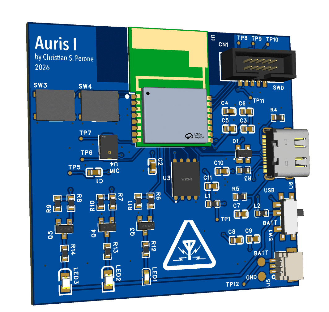
This short article is just to share a new side project I started working on during the 2025/2026 break. Over the past year, we have started to see a vast number of companies developing hardware for AI assistants. There were also a lot of acquisitions related to these devices (e.g., Amazon bought Bee [1]), and there were also a lot of fiascos, of course (e.g., Rabbit devices, Humane, and so on). I think that these devices have a strong future ahead due to their potential, so I started prototyping some code for recording, compression, and transmission, and testing some microphones. I found excellent transcription results even with a single microphone, so I decided to start a small side project which ended up becoming the the Auris I on the right.
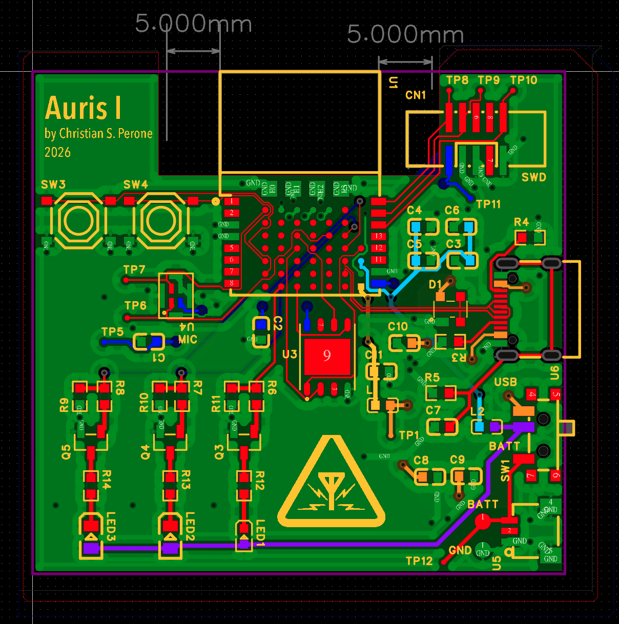
Routing took quite a bit of work, as the main SoC used not only castellated pins but also pins under the chip which were very difficult to route. Another issue was the requirements of the RF module, which required some clearance on the ground plane, however, this was still much easier than going straight with the RF SoC without the guest board. The main challenges now are chip shortages for some components, but I expect to have a prototype working by the end of February. I will do another post then with more details and some interesting results. The board ended up being only 5 cm. There is, of course, a lot that can be reduced, but that will come in the Auris II after I manage to hack it a bit.
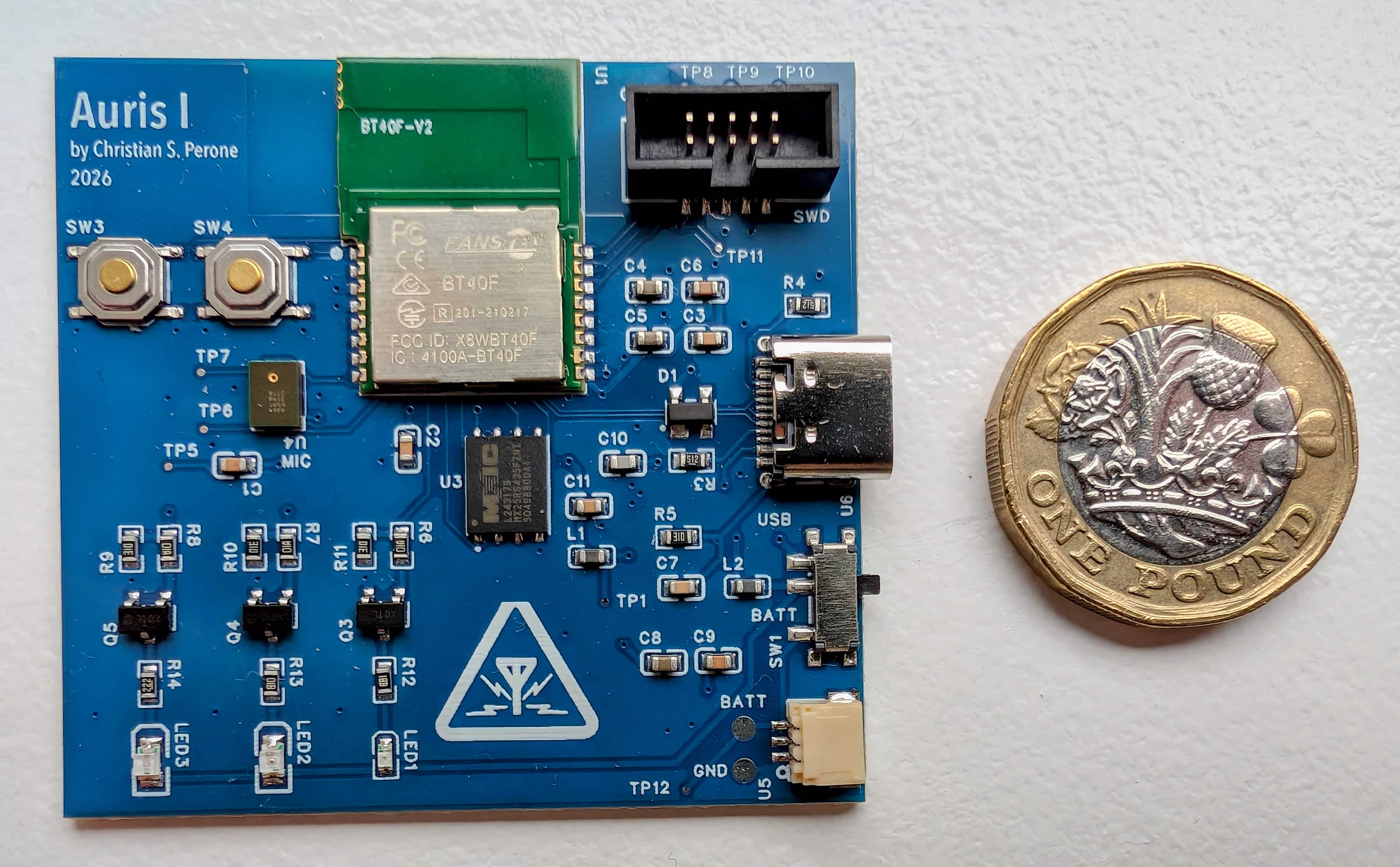
Update 7/Feb: Manufacturing, PCBs arrived !
I decided to go with JLCPCB with 4 layers as it is often quick and also very cheap, the only issue I faced was with the components, my board is based on nRF5340 (from Nordic Semiconductor) and modules with it were all without stock, so I had to acquire and wait for them to ship to JLCPCB, which took around 2 weeks. After that it was another week for the PCB fabrication and the assembly as well. Since the MEMS microphone was so small and the nRF5340 module also had pads under it, they required an x-ray inspection to make sure it was all connected fine. But that was around 4 pounds for x-ray and it was very fast as well. After around 5 days in total I finally received the PCBs and the quality is just amazing, I didn’t even order the cleaning of the board but they came all very clean well soldered as well.
I did all tests for the external flash, microphone, leds, battery/usb supply and also the SWD connection and it is all working fine, so now it is the fun part of coding, soon I will open-source everything, so stay tuned !
– Christian S. Perone
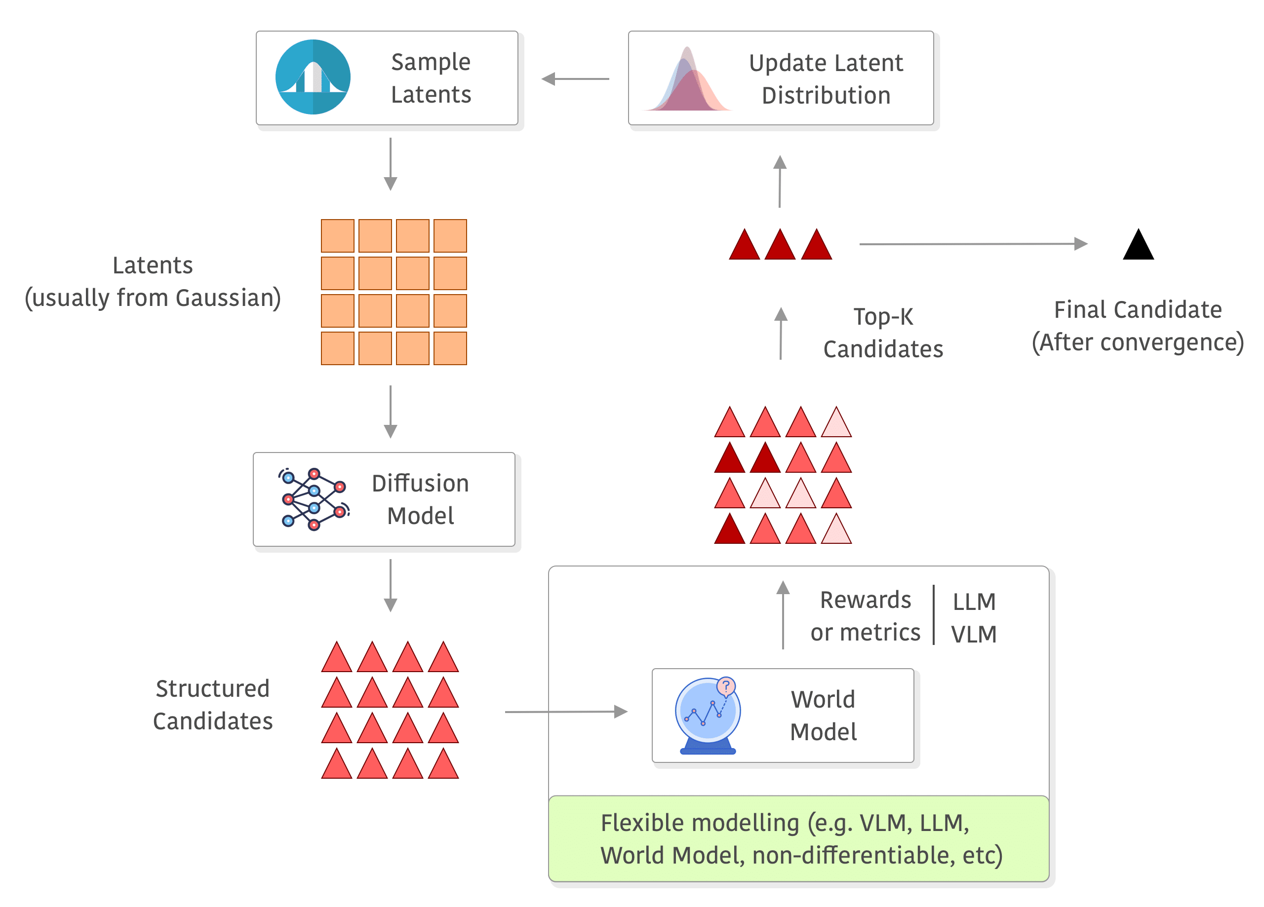
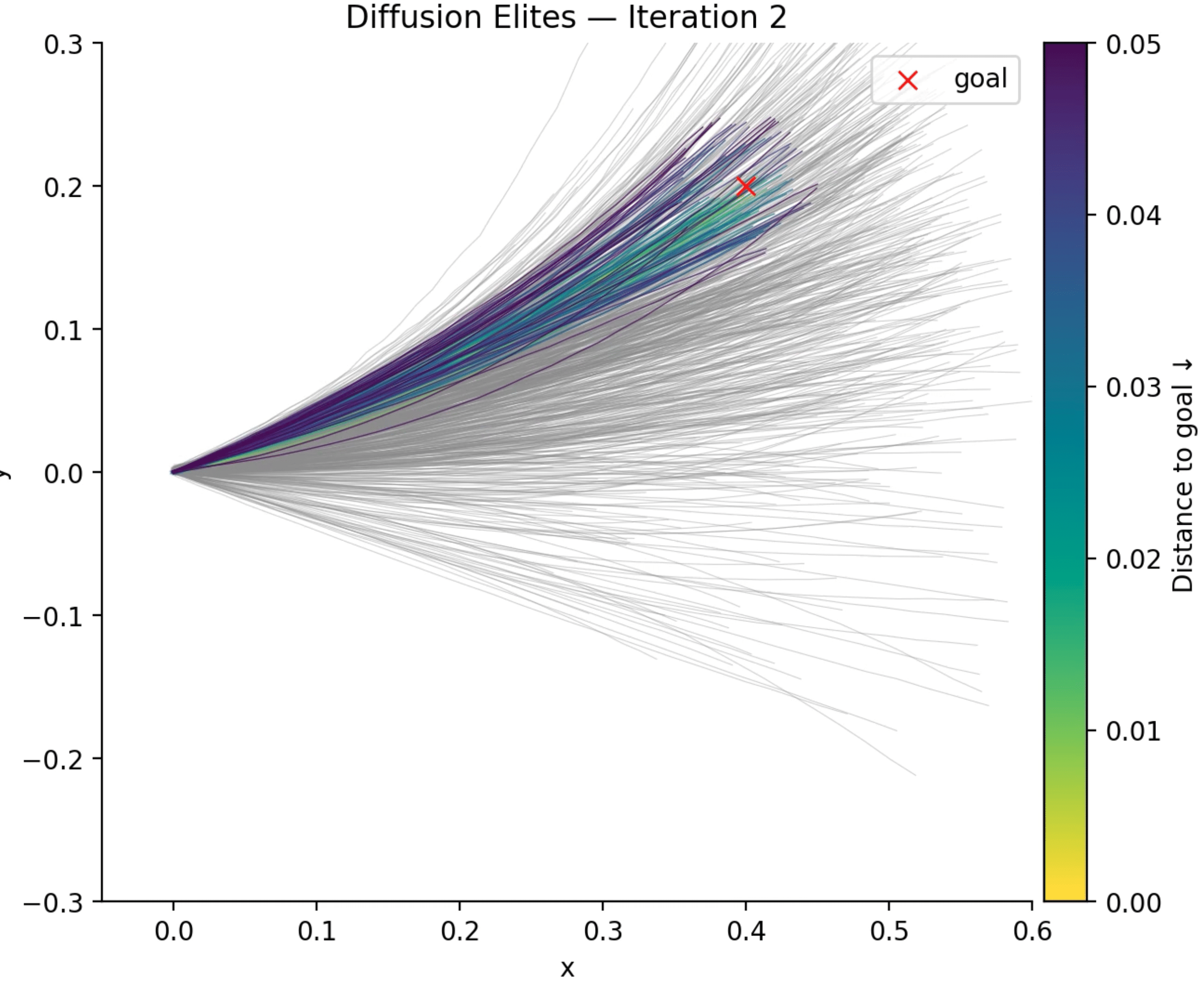 It is not a secret that Diffusion models have become the workhorses of high-dimensionality generation: start with a Gaussian noise and, through a learned denoising trajectory, you get high-fidelity images, molecular graphs, or robot trajectories that look (uncannily) real. I wrote extensively about diffusion and its connection with the