Short animation showing the ICU occupancy forecasting for Portugal during the COVID-19 outbreak. For more information, visit the site below:
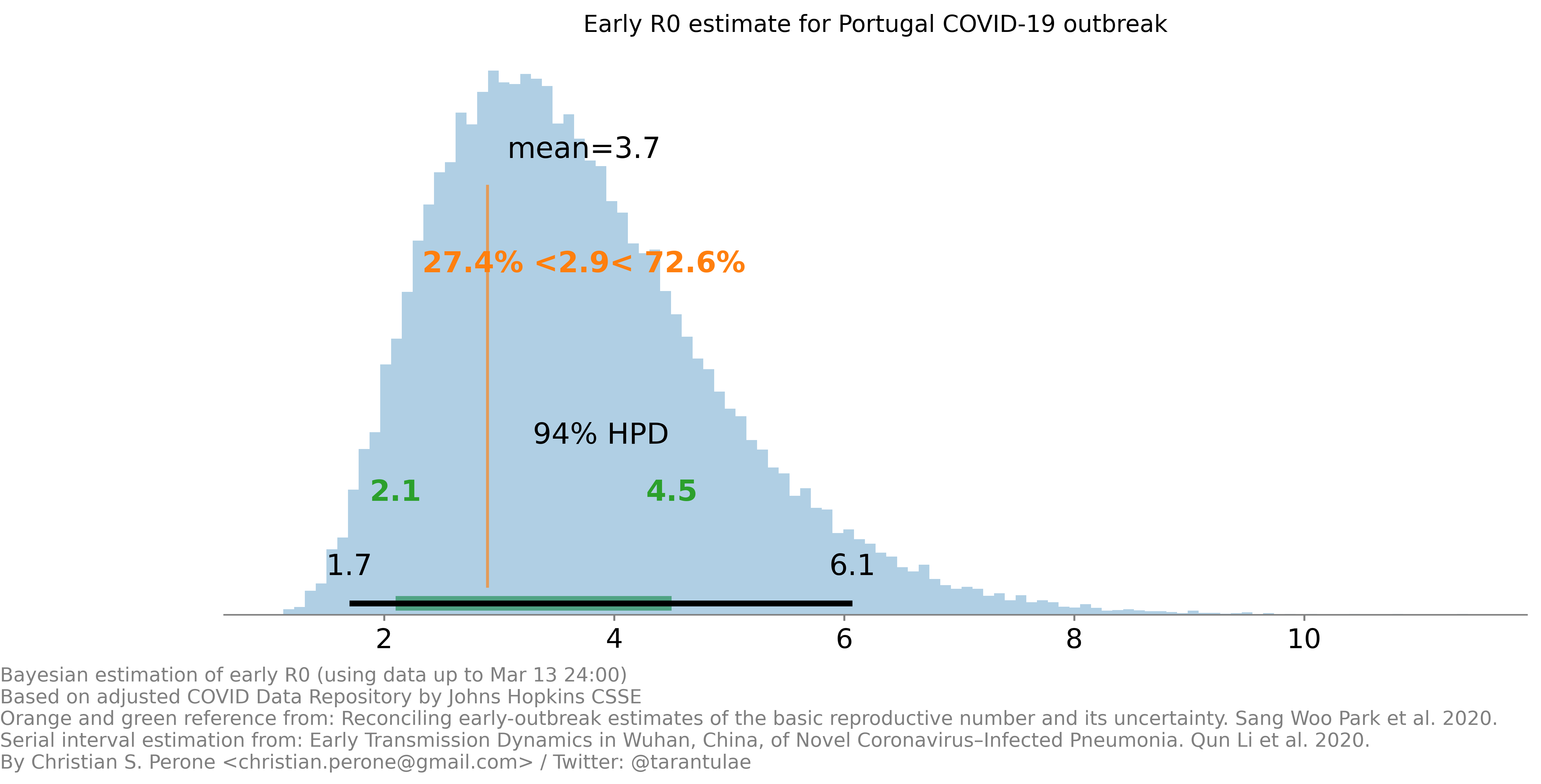
Just posting the first early estimate for the COVID-19 
Cite this article as: Christian S. Perone, "First early R0 estimate for Portugal COVID-19 outbreak," in Terra Incognita, 14/03/2020, https://blog.christianperone.com/2020/03/first-early-r0-estimate-for-portugal-covid-19-outbreak/.
Since the generation time of a virus is very difficult to estimate, most studies rely on the serial interval which is estimated from the interval between clinical onsets. Given that most analysis use the serial interval, it is paramount to have an estimate of the precise onset dates of the symptoms.
I did a analysis for all states in Brazil using data from SIVEP-Gripe, the complete analysis is available here.
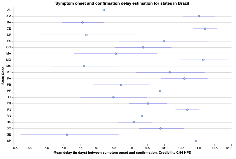
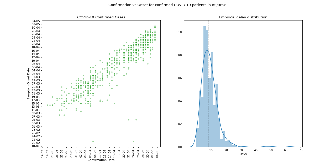
In the image above, we can see the gamma mean estimate for the delay on each state in Brazil. Below you can see the distribution for Rio Grande do Sul / RS:
Introduction
This is the post of 2020, so happy new year to you all !
I’m a huge fan of LLVM since 11 years ago when I started playing with it to JIT data structures such as AVLs, then later to JIT restricted AST trees and to JIT native code from TensorFlow graphs. Since then, LLVM evolved into one of the most important compiler framework ecosystem and is used nowadays by a lot of important open-source projects.
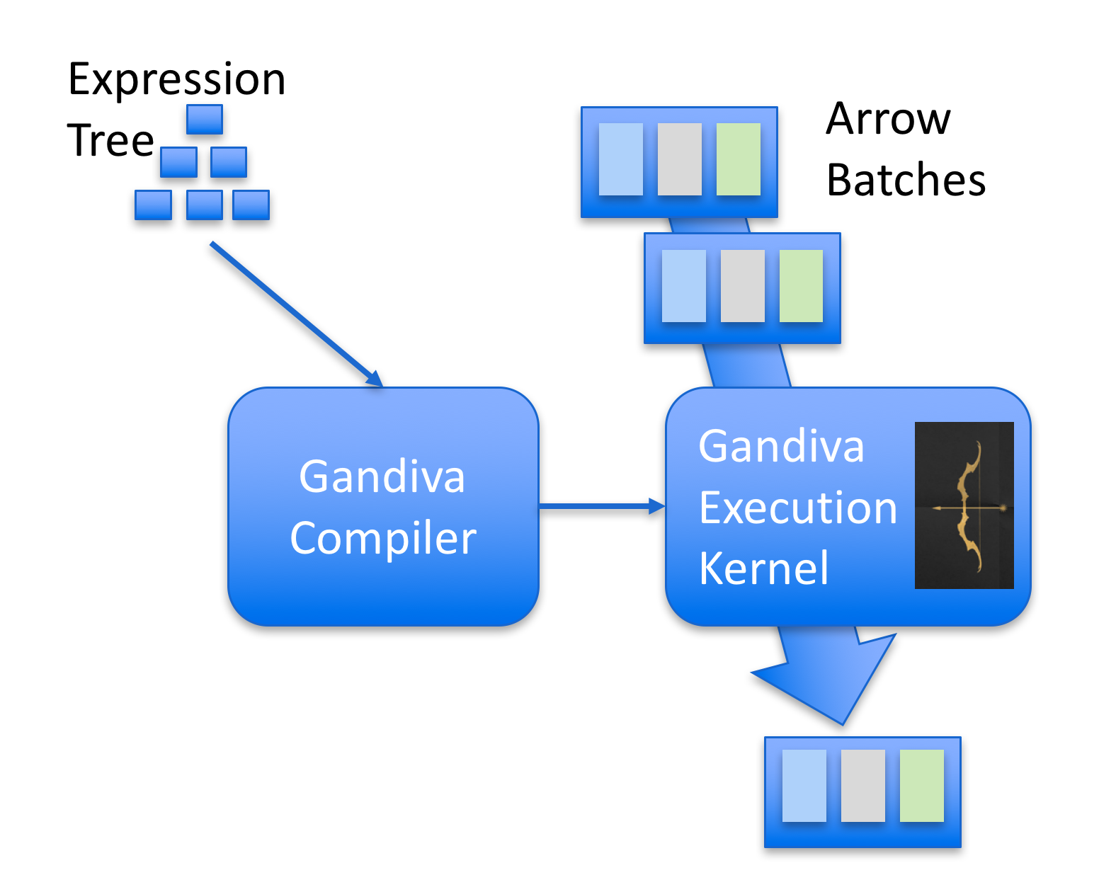
One cool project that I recently became aware of is Gandiva. Gandiva was developed by Dremio and then later donated to Apache Arrow (kudos to Dremio team for that). The main idea of Gandiva is that it provides a compiler to generate LLVM IR that can operate on batches of Apache Arrow. Gandiva was written in C++ and comes with a lot of different functions implemented to build an expression tree that can be JIT’ed using LLVM. One nice feature of this design is that it can use LLVM to automatically optimize complex expressions, add native target platform vectorization such as AVX while operating on Arrow batches and execute native code to evaluate the expressions.
The image below gives an overview of Gandiva:
In this post I’ll build a very simple expression parser supporting a limited set of operations that I will use to filter a Pandas DataFrame.
Building simple expression with Gandiva
In this section I’ll show how to create a simple expression manually using tree builder from Gandiva.
Using Gandiva Python bindings to JIT and expression
Before building our parser and expression builder for expressions, let’s manually build a simple expression with Gandiva. First, we will create a simple Pandas DataFrame with numbers from 0.0 to 9.0:
import pandas as pd
import pyarrow as pa
import pyarrow.gandiva as gandiva

# Create a simple Pandas DataFrame
df = pd.DataFrame({"x": [1.0 * i for i in range(10)]})
table = pa.Table.from_pandas(df)
schema = pa.Schema.from_pandas(df)
We converted the DataFrame to an Arrow Table, it is important to note that in this case it was a zero-copy operation, Arrow isn’t copying data from Pandas and duplicating the DataFrame. Later we get the schemafrom the table, that contains column types and other metadata.
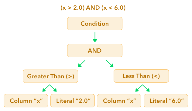
After that, we want to use Gandiva to build the following expression to filter the data:
(x > 2.0) and (x < 6.0)
This expression will be built using nodes from Gandiva:
builder = gandiva.TreeExprBuilder()

# Reference the column "x"
node_x = builder.make_field(table.schema.field("x"))

# Make two literals: 2.0 and 6.0
two = builder.make_literal(2.0, pa.float64())
six = builder.make_literal(6.0, pa.float64())

# Create a function for "x > 2.0"
gt_five_node = builder.make_function("greater_than",
                                     [node_x, two],
                                     pa.bool_())

# Create a function for "x < 6.0"
lt_ten_node = builder.make_function("less_than",
                                    [node_x, six],
                                    pa.bool_())
# Create an "and" node, for "(x > 2.0) and (x < 6.0)"
and_node = builder.make_and([gt_five_node, lt_ten_node])

# Make the expression a condition and create a filter
condition = builder.make_condition(and_node)
filter_ = gandiva.make_filter(table.schema, condition)
This code now looks a little more complex but it is easy to understand. We are basically creating the nodes of a tree that will represent the expression we showed earlier. Here is a graphical representation of what it looks like:
Inspecting the generated LLVM IR
Unfortunately, haven’t found a way to dump the LLVM IR that was generated using the Arrow’s Python bindings, however, we can just use the C++ API to build the same tree and then look at the generated LLVM IR:
auto field_x = field("x", float32());
auto schema = arrow::schema({field_x});

auto node_x = TreeExprBuilder::MakeField(field_x);

auto two = TreeExprBuilder::MakeLiteral((float_t)2.0);
auto six = TreeExprBuilder::MakeLiteral((float_t)6.0);

auto gt_five_node = TreeExprBuilder::MakeFunction("greater_than",
                                                  {node_x, two}, arrow::boolean());

auto lt_ten_node = TreeExprBuilder::MakeFunction("less_than",
                                                 {node_x, six}, arrow::boolean());

auto and_node = TreeExprBuilder::MakeAnd({gt_five_node, lt_ten_node});
auto condition = TreeExprBuilder::MakeCondition(and_node);

std::shared_ptr<Filter> filter;
auto status = Filter::Make(schema, condition, TestConfiguration(), &filter);
The code above is the same as the Python code, but using the C++ Gandiva API. Now that we built the tree in C++, we can get the LLVM Module and dump the IR code for it. The generated IR is full of boilerplate code and the JIT’ed functions from the Gandiva registry, however the important parts are show below:
; Function Attrs: alwaysinline norecurse nounwind readnone ssp uwtable
define internal zeroext i1 @less_than_float32_float32(float, float) local_unnamed_addr #0 {
  %3 = fcmp olt float %0, %1
  ret i1 %3
}

; Function Attrs: alwaysinline norecurse nounwind readnone ssp uwtable
define internal zeroext i1 @greater_than_float32_float32(float, float) local_unnamed_addr #0 {
  %3 = fcmp ogt float %0, %1
  ret i1 %3
}

(...)
%x = load float, float* %11
%greater_than_float32_float32 = call i1 @greater_than_float32_float32(float %x, float 2.000000e+00)
(...)
%x11 = load float, float* %15
%less_than_float32_float32 = call i1 @less_than_float32_float32(float %x11, float 6.000000e+00)
As you can see, on the IR we can see the call to the functions less_than_float32_float_32 and greater_than_float32_float32that are the (in this case very simple) Gandiva functions to do float comparisons. Note the specialization of the function by looking at the function name prefix.
What is quite interesting is that LLVM will apply all optimizations in this code and it will generate efficient native code for the target platform while Godiva and LLVM will take care of making sure that memory alignment will be correct for extensions such as AVX to be used for vectorization.
This IR code I showed isn’t actually the one that is executed, but the optimized one. And in the optimized one we can see that LLVM inlined the functions, as shown in a part of the optimized code below:
%x.us = load float, float* %10, align 4
%11 = fcmp ogt float %x.us, 2.000000e+00
%12 = fcmp olt float %x.us, 6.000000e+00
%not.or.cond = and i1 %12, %11
You can see that the expression is now much simpler after optimization as LLVM applied its powerful optimizations and inlined a lot of Gandiva funcions.
Building a Pandas filter expression JIT with Gandiva
Now we want to be able to implement something similar as the Pandas’ DataFrame.query()function using Gandiva. The first problem we will face is that we need to parse a string such as (x > 2.0) and (x < 6.0), later we will have to build the Gandiva expression tree using the tree builder from Gandiva and then evaluate that expression on arrow data.
Now, instead of implementing a full parsing of the expression string, I’ll use the Python AST module to parse valid Python code and build an Abstract Syntax Tree (AST) of that expression, that I’ll be later using to emit the Gandiva/LLVM nodes.
The heavy work of parsing the string will be delegated to Python AST module and our work will be mostly walking on this tree and emitting the Gandiva nodes based on that syntax tree. The code for visiting the nodes of this Python AST tree and emitting Gandiva nodes is shown below:
class LLVMGandivaVisitor(ast.NodeVisitor):
    def __init__(self, df_table):
        self.table = df_table
        self.builder = gandiva.TreeExprBuilder()
        self.columns = {f.name: self.builder.make_field(f)
                        for f in self.table.schema}
        self.compare_ops = {
            "Gt": "greater_than",
            "Lt": "less_than",
        }
        self.bin_ops = {
            "BitAnd": self.builder.make_and,
            "BitOr": self.builder.make_or,
        }

    def visit_Module(self, node):
        return self.visit(node.body[0])

    def visit_BinOp(self, node):
        left = self.visit(node.left)
        right = self.visit(node.right)
        op_name = node.op.__class__.__name__
        gandiva_bin_op = self.bin_ops[op_name]
        return gandiva_bin_op([left, right])

    def visit_Compare(self, node):
        op = node.ops[0]
        op_name = op.__class__.__name__
        gandiva_comp_op = self.compare_ops[op_name]
        comparators = self.visit(node.comparators[0])
        left = self.visit(node.left)
        return self.builder.make_function(gandiva_comp_op,
                                          [left, comparators], pa.bool_())

    def visit_Num(self, node):
        return self.builder.make_literal(node.n, pa.float64())

    def visit_Expr(self, node):
        return self.visit(node.value)

    def visit_Name(self, node):
        return self.columns[node.id]

    def generic_visit(self, node):
        return node

    def evaluate_filter(self, llvm_mod):
        condition = self.builder.make_condition(llvm_mod)
        filter_ = gandiva.make_filter(self.table.schema, condition)
        result = filter_.evaluate(self.table.to_batches()[0],
                                  pa.default_memory_pool())
        arr = result.to_array()
        pd_result = arr.to_numpy()
        return pd_result

    @staticmethod
    def gandiva_query(df, query):
        df_table = pa.Table.from_pandas(df)
        llvm_gandiva_visitor = LLVMGandivaVisitor(df_table)
        mod_f = ast.parse(query)
        llvm_mod = llvm_gandiva_visitor.visit(mod_f)
        results = llvm_gandiva_visitor.evaluate_filter(llvm_mod)
        return results
As you can see, the code is pretty straightforward as I’m not supporting every possible Python expressions but a minor subset of it. What we do in this class is basically a conversion of the Python AST nodes such as Comparators and BinOps (binary operations) to the Gandiva nodes. I’m also changing the semantics of the & and the | operators to represent AND and OR respectively, such as in Pandas query()function.
Register as a Pandas extension
The next step is to create a simple Pandas extension using the gandiva_query() method that we created:
@pd.api.extensions.register_dataframe_accessor("gandiva")
class GandivaAcessor:
    def __init__(self, pandas_obj):
        self.pandas_obj = pandas_obj

    def query(self, query):
         return LLVMGandivaVisitor.gandiva_query(self.pandas_obj, query)
And that is it, now we can use this extension to do things such as:
df = pd.DataFrame({"a": [1.0 * i for i in range(nsize)]})
results = df.gandiva.query("a > 10.0")
As we have registered a Pandas extension called gandiva that is now a first-class citizen of the Pandas DataFrames.
Let’s create now a 5 million floats DataFrame and use the new query() method to filter it:
df = pd.DataFrame({"a": [1.0 * i for i in range(50000000)]})
df.gandiva.query("a < 4.0")

# This will output:
#     array([0, 1, 2, 3], dtype=uint32)
Note that the returned values are the indexes satisfying the condition we implemented, so it is different than the Pandas query()that returns the data already filtered.
I did some benchmarks and found that Gandiva is usually always faster than Pandas, however I’ll leave proper benchmarks for a next post on Gandiva as this post was to show how you can use it to JIT expressions.
That’s it ! I hope you liked the post as I enjoyed exploring Gandiva. It seems that we will probably have more and more tools coming up with Gandiva acceleration, specially for SQL parsing/projection/JITing. Gandiva is much more than what I just showed, but you can get started now to understand more of its architecture and how to build the expression trees.
– Christian S. Perone
Cite this article as: Christian S. Perone, "Gandiva, using LLVM and Arrow to JIT and evaluate Pandas expressions," in Terra Incognita, 19/01/2020, https://blog.christianperone.com/2020/01/gandiva-using-llvm-and-arrow-to-jit-and-evaluate-pandas-expressions/.
Training neural networks is often done by measuring many different metrics such as accuracy, loss, gradients, etc. This is most of the time done aggregating these metrics and plotting visualizations on TensorBoard.
 There are, however, other senses that we can use to monitor the training of neural networks, such as sound. Sound is one of the perspectives that is currently very poorly explored in the training of neural networks. Human hearing can be very good a distinguishing very small perturbations in characteristics such as rhythm and pitch, even when these perturbations are very short in time or subtle.
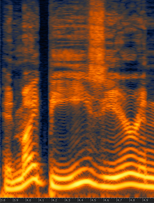
For this experiment, I made a very simple example showing a synthesized sound that was made using the gradient norm of each layer and for step of the training for a convolutional neural network training on MNIST using different settings such as different learning rates, optimizers, momentum, etc.
You’ll need to install PyAudio and PyTorch to run the code (in the end of this post).
Training sound with SGD using LR 0.01
This segment represents a training session with gradients from 4 layers during the first 200 steps of the first epoch and using a batch size of 10. The higher the pitch, the higher the norm for a layer, there is a short silence to indicate different batches. Note the gradient increasing during time.
Training sound with SGD using LR 0.1
Same as above, but with higher learning rate.
Training sound with SGD using LR 1.0
Same as above, but with high learning rate that makes the network to diverge, pay attention to the high pitch when the norms explode and then divergence.
Training sound with SGD using LR 1.0 and BS 256
Same setting but with a high learning rate of 1.0 and a batch size of 256. Note how the gradients explode and then there are NaNs causing the final sound.
Training sound with Adam using LR 0.01
This is using Adam in the same setting as the SGD.
Source code
For those who are interested, here is the entire source code I used to make the sound clips:
import pyaudio
import numpy as np
import wave

import torch
import torch.nn as nn
import torch.nn.functional as F
import torch.optim as optim
from torchvision import datasets, transforms


class Net(nn.Module):
    def __init__(self):
        super(Net, self).__init__()
        self.conv1 = nn.Conv2d(1, 20, 5, 1)
        self.conv2 = nn.Conv2d(20, 50, 5, 1)
        self.fc1 = nn.Linear(4*4*50, 500)
        self.fc2 = nn.Linear(500, 10)

        self.ordered_layers = [self.conv1,
                               self.conv2,
                               self.fc1,
                               self.fc2]

    def forward(self, x):
        x = F.relu(self.conv1(x))
        x = F.max_pool2d(x, 2, 2)
        x = F.relu(self.conv2(x))
        x = F.max_pool2d(x, 2, 2)
        x = x.view(-1, 4*4*50)
        x = F.relu(self.fc1(x))
        x = self.fc2(x)
        return F.log_softmax(x, dim=1)


def open_stream(fs):
    p = pyaudio.PyAudio()
    stream = p.open(format=pyaudio.paFloat32,
                    channels=1,
                    rate=fs,
                    output=True)
    return p, stream


def generate_tone(fs, freq, duration):
    npsin = np.sin(2 * np.pi * np.arange(fs*duration) * freq / fs)
    samples = npsin.astype(np.float32)
    return 0.1 * samples


def train(model, device, train_loader, optimizer, epoch):
    model.train()

    fs = 44100
    duration = 0.01
    f = 200.0
    p, stream = open_stream(fs)

    frames = []

    for batch_idx, (data, target) in enumerate(train_loader):
        data, target = data.to(device), target.to(device)
        optimizer.zero_grad()
        output = model(data)
        loss = F.nll_loss(output, target)
        loss.backward()

        norms = []
        for layer in model.ordered_layers:
            norm_grad = layer.weight.grad.norm()
            norms.append(norm_grad)

            tone = f + ((norm_grad.numpy()) * 100.0)
            tone = tone.astype(np.float32)
            samples = generate_tone(fs, tone, duration)

            frames.append(samples)

        silence = np.zeros(samples.shape[0] * 2,
                           dtype=np.float32)
        frames.append(silence)

        optimizer.step()

        # Just 200 steps per epoach
        if batch_idx == 200:
            break

    wf = wave.open("sgd_lr_1_0_bs256.wav", 'wb')
    wf.setnchannels(1)
    wf.setsampwidth(p.get_sample_size(pyaudio.paFloat32))
    wf.setframerate(fs)
    wf.writeframes(b''.join(frames))
    wf.close()

    stream.stop_stream()
    stream.close()
    p.terminate()


def run_main():
    device = torch.device("cpu")

    train_loader = torch.utils.data.DataLoader(
        datasets.MNIST('../data', train=True, download=True,
                       transform=transforms.Compose([
                           transforms.ToTensor(),
                           transforms.Normalize((0.1307,), (0.3081,))
                       ])),
        batch_size=256, shuffle=True)

    model = Net().to(device)
    optimizer = optim.SGD(model.parameters(), lr=0.01, momentum=0.5)

    for epoch in range(1, 2):
        train(model, device, train_loader, optimizer, epoch)


if __name__ == "__main__":
    run_main()
Cite this article as: Christian S. Perone, "Listening to the neural network gradient norms during training," in Terra Incognita, 04/08/2019, https://blog.christianperone.com/2019/08/listening-to-the-neural-network-gradient-norms-during-training/.
A few months ago I made a post about Randomized Prior Functions for Deep Reinforcement Learning, where I showed how to implement the training procedure in PyTorch and how to extract the model uncertainty from them.
Using the same code showed earlier, these animations below show the training of an ensemble of 40 models with 2-layer MLP and 20 hidden units in different settings. These visualizations are really nice to understand what are the convergence differences when using or not bootstrap or randomized priors.
Naive Ensemble
This is a training session without bootstrapping data or adding a randomized prior, it’s just a naive ensembling:
Ensemble with Randomized Prior
This is the ensemble but with the addition of the randomized prior (MLP with the same architecture, with random weights and fixed):
$$Q_{\theta_k}(x) = f_{\theta_k}(x) + p_k(x)$$
The final model \(Q_{\theta_k}(x)\) will be the k model of the ensemble that will fit the function \(f_{\theta_k}(x)\) with an untrained prior \(p_k(x)\):
Ensemble with Randomized Prior and Bootstrap
This is a ensemble with the randomized prior functions and data bootstrap:
Ensemble with a fixed prior and bootstrapping
This is an ensemble with a fixed prior (Sin) and bootstrapping:
Cite this article as: Christian S. Perone, "Visualizing network ensembles with bootstrap and randomized priors," in Terra Incognita, 20/07/2019, https://blog.christianperone.com/2019/07/visualizing-network-ensembles-with-bootstrap-and-randomized-priors/.
Introduction
Not a lot of people working with the Python scientific ecosystem are aware of the NEP 18 (dispatch mechanism for NumPy’s high-level array functions). Given the importance of this protocol, I decided to write this short introduction to the new dispatcher that will certainly bring a lot of benefits for the Python scientific ecosystem.
If you used PyTorch, TensorFlow, Dask, etc, you certainly noticed the similarity of their API contracts with Numpy. And it’s not by accident, Numpy’s API is one of the most fundamental and widely-used APIs for scientific computing. Numpy is so pervasive, that it ceased to be only an API and it is becoming more a protocol or an API specification.
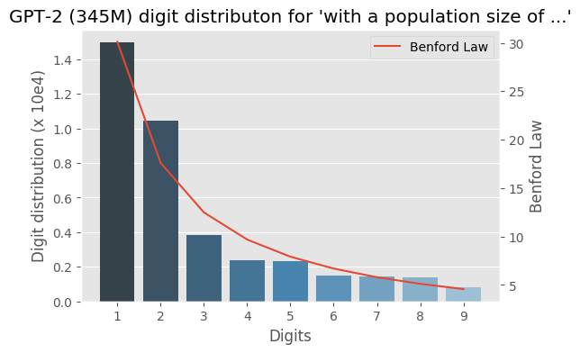
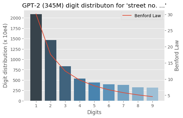
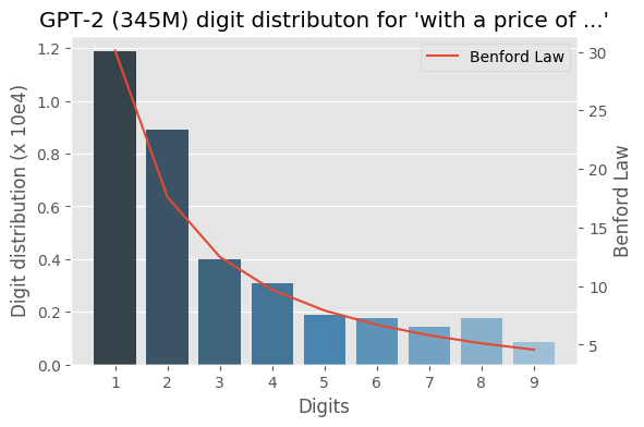
I wrote some months ago about how the Benford law emerges from language models, today I decided to evaluate the same method to check how the GPT-2 would behave with some sentences and it turns out that it seems that it is also capturing these power laws. You can find some plots with the examples below, the plots are showing the probability of the digit given a particular sentence such as “with a population size of”, showing the distribution of: $$P(\{1,2, \ldots, 9\} \vert \text{“with a population size of”})$$ for the GPT-2 medium model (345M):
Cite this article as: Christian S. Perone, "Benford law on GPT-2 language model," in Terra Incognita, 14/06/2019, https://blog.christianperone.com/2019/06/benford-law-on-gpt-2-language-model/.