Hoje finalmente consegui rastrear um dos balões meteorológicos que a aeronáutica lança duas vezes por dia aqui em Porto Alegre / RS. A aeronáutica utiliza as sondas da Vaisala (uma empresa finlandesa) modelo RS-92SGP para realizar as medições de umidade, temperatura e pressão. Estes dados são geralmente utilizados para as previsões de tempo da região; existe um datasheet com mais dados sobre o equipamento que eles utilizam, neste datasheet tem informações importantes como por exemplo a frequência em que o aparelho envia os dados de telemetria. Aqui em Porto Alegre / RS a aeronáutica está utilizando a faixa de operação em 402.700Mhz, que também é coberta pelos dongles USB RTLSDR como o que eu utilizo.
O equipamento da Vaisala é um equipamento que utiliza 60mW de potência na transmissão (eu já vi balões transmitindo até 600km nessa frequência com apenas 10mW e com uma antena decente é claro) e utiliza modulação GFSK. Para decodificar o protocolo e GFSK podemos utilizar SDR# juntamente com o Virtual Cable (ou algo semelhante para redirecionar os dados do SDR# para o SondeMonitor que é o software que irá fazer a decodificação dos dados (infelizmente o software é pag e só roda apenas em Windows, mas ao menos vem com alguns dias de trial).
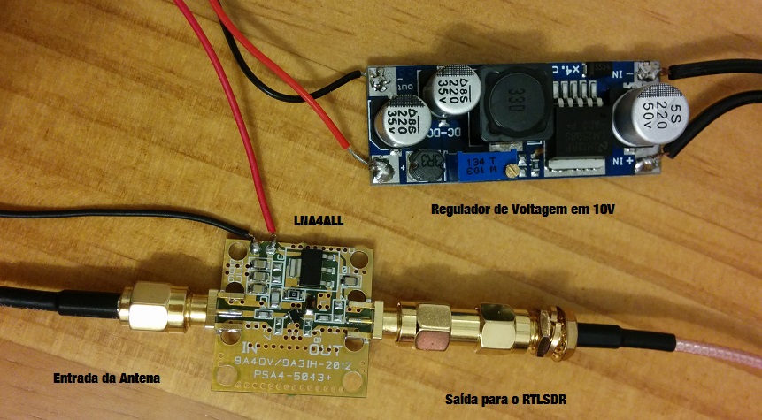
No meu setup eu estou utilizando um dongle RTLSDR R820T juntamente com um Low Noise Amplifier (LNA4ALL na foto abaixo) e uma antena de 5dB omnidirecional:
LNA e regulador de tensão
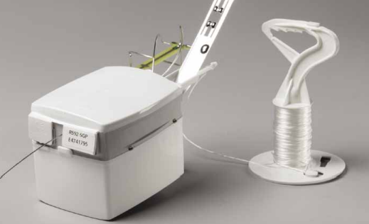
Abaixo segue a foto do equipamento lançado como payload do balão meteorológico:
Sonda RS92-SGP
Estes balões geralmente atingem uma altitude de uns 20km a 35km, mas isto depende de vários fatores como por exemplo os ventos, a quantidade de gás que foi utilizada no balão, a espessura do latex do balão e outros fatores. Quando o balão estoura este fenômeno é geralmente chamado de “burst” e após este estouro o balão acaba caindo por terra (ele tem uma bateria que não agride a natureza).
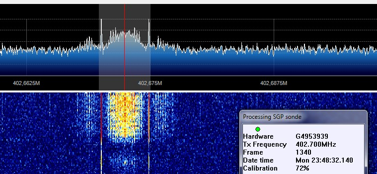
Seguem abaixo os screenshots do recebimento dos dados, neste momento eu ainda não havia conseguido receber toda calibração do aparelho:
SDR# recebendo o sinal da sonda
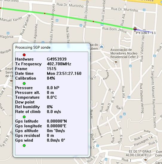
Screenshot de alguém mais fazendo o tracking da sonda e jogando para o APRS aqui de Porto Alegre:
Localização do balão no APRS
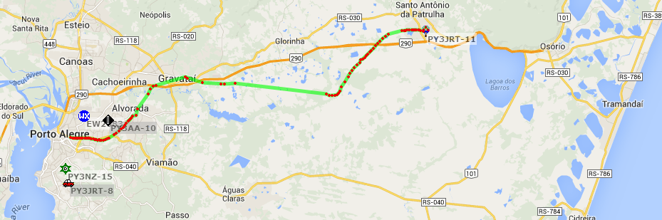
Imagem do rastremento do balão no APRS:
O próximo passo agora é conseguir uma antena direcional para melhorar a recepção =)
Para quem tiver interesse em receber os dados, os balões são lançados diariamente as 00:00 UTC e às 12:00 UTC.
The new generation of OpenCV bindings for Python is getting better and better with the hard work of the community. The new bindings, called “cv2” are the replacement of the old “cv” bindings; in this new generation of bindings, almost all operations returns now native Python objects or Numpy objects, which is pretty nice since it simplified a lot and also improved performance on some areas due to the fact that you can now also use the optimized operations from Numpy and also enabled the integration with other frameworks like the scikit-image which also uses Numpy arrays for image representation.
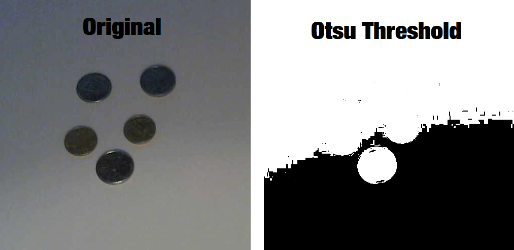
In this example, I’ll show how to segment coins present in images or even real-time video capture with a simple approach using thresholding, morphological operators, and contour approximation. This approach is a lot simpler than the approach using Otsu’s thresholding and Watershed segmentation here in OpenCV Python tutorials, which I highly recommend you to read due to its robustness. Unfortunately, the approach using Otsu’s thresholding is highly dependent on an illumination normalization. One could extract small patches of the image to implement something similar to an adaptive Otsu’s binarization (like the one implemented in Letptonica – the framework used by Tesseract OCR) to overcome this problem, but let’s see another approach. For reference, see the output of the Otsu’s thresholding using an image taken with my webcam with a non-normalized illumination:
Original image vs Otsu binarization
1. Setting the Video Capture configuration
The first step to create a real-time Video Capture using the Python bindings is to instantiate the VideoCapture class, set the properties and then start reading frames from the camera:
import numpy as np
import cv2

cap = cv2.VideoCapture(0)
cap.set(cv2.cv.CV_CAP_PROP_FRAME_WIDTH, 1280)
cap.set(cv2.cv.CV_CAP_PROP_FRAME_HEIGHT, 720)
In newer versions (unreleased yet), the constants for CV_CAP_PROP_FRAME_WIDTH are now in the cv2 module, for now, let’s just use the cv2.cv module.
2. Reading image frames
The next step is to use the VideoCapture object to read the frames and then convert them to gray color (we are not going to use color information to segment the coins):
while True:
    ret, frame = cap.read()
    roi = frame[0:500, 0:500]
    gray = cv2.cvtColor(roi, cv2.COLOR_BGR2GRAY)
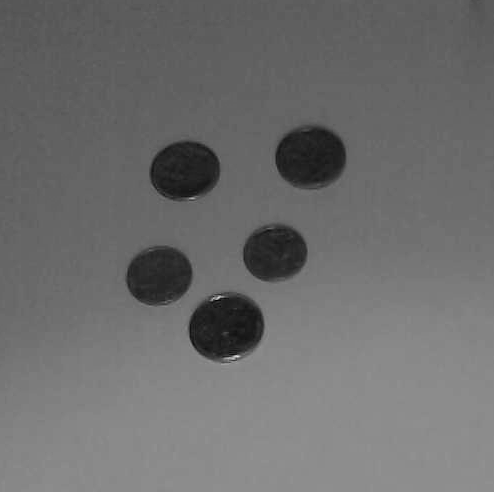
Note that here I’m extracting a small portion of the complete image (where the coins are located), but you don’t have to do that if you have only coins on your image. At this moment, we have the following gray image:
The original Gray image captured.
3. Applying adaptive thresholding
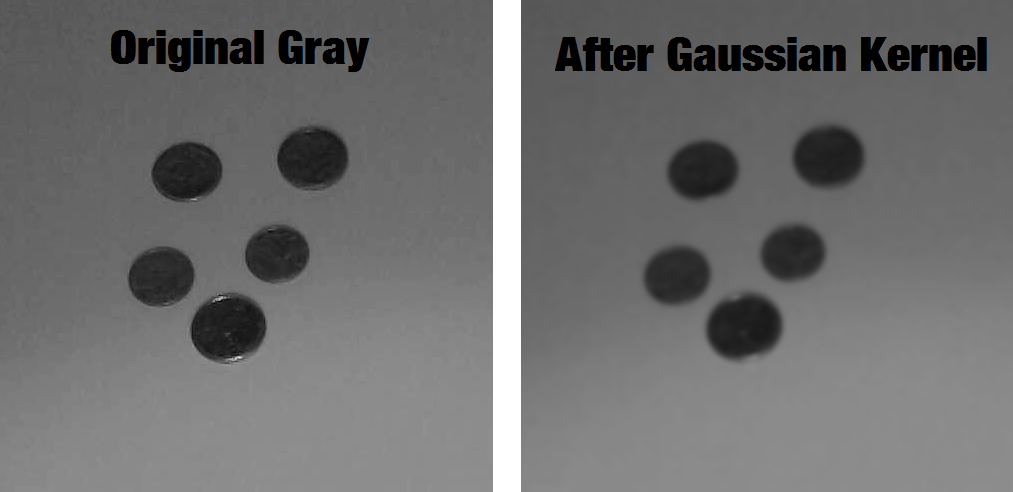
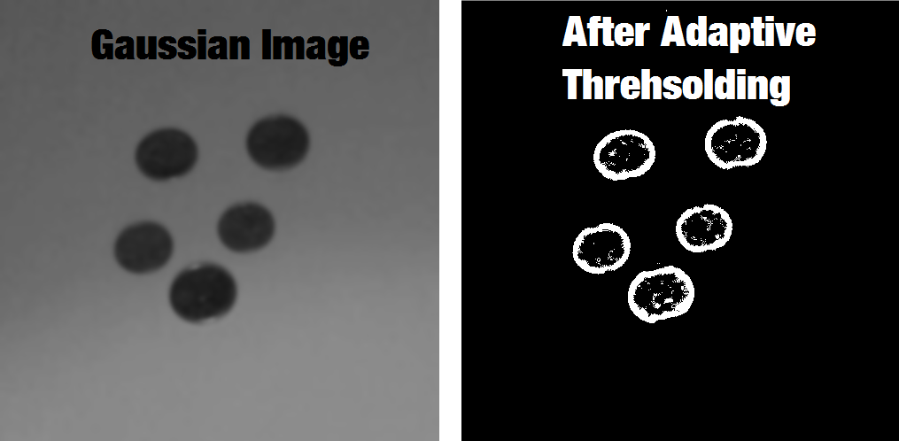
In this step we will apply the Adaptive Thresholding after applying a Gaussian Blur kernel to eliminate the noise that we have in the image:
See the effect of the Gaussian Kernel in the image:
The original gray image and the image after applying the Gaussian Kernel.
And now the effect of the Adaptive Thresholding with the blurry image:
Note that at that moment we already have the coins segmented except for the small noisy inside the center of the coins and also in some places around them.
4. Morphology
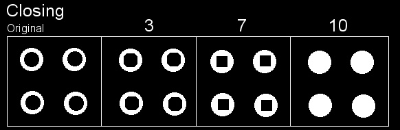
The Morphological Operators are used to dilate, erode and other operations on the pixels of the image. Here, due to the fact that sometimes the camera can present some artifacts, we will use the Morphological Operation of Closing to make sure that the borders of the coins are always close, otherwise, we may found a coin with a semi-circle or something like that. To understand the effect of the Closing operation (which is the operation of erosion of the pixels already dilated) see the image below:
You can see that after some iterations of the operation, the circles start to become filled. To use the Closing operation, we’ll use the morphologyEx function from the OpenCV Python bindings:
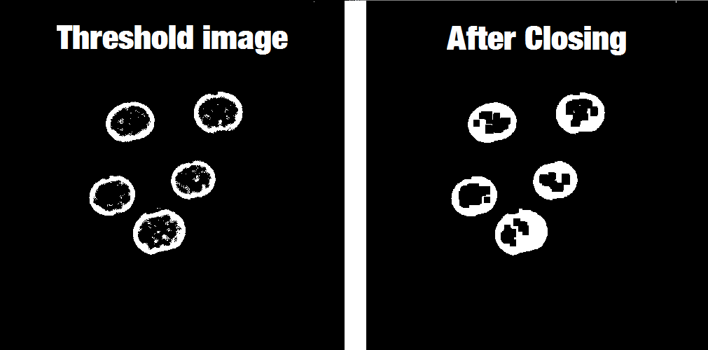
See now the effect of the Closing operation on our coins:
The operations of Morphological Operators are very simple, the main principle is the application of an element (in our case we have a block element of 3×3) into the pixels of the image. If you want to understand it, please see this animation explaining the operation of Erosion.
5. Contour detection and filtering
After applying the morphological operators, all we have to do is to find the contour of each coin and then filter the contours having an area smaller or larger than a coin area. You can imagine the procedure of finding contours in OpenCV as the operation of finding connected components and their boundaries. To do that, we’ll use the OpenCV findContours function.
Note that we made a copy of the closing image because the function findContours will change the image passed as the first parameter, we’re also using the RETR_EXTERNAL flag, which means that the contours returned are only the extreme outer contours. The parameter CHAIN_APPROX_SIMPLE will also return a compact representation of the contour, for more information see here.
After finding the contours, we need to iterate into each one and check the area of them to filter the contours containing an area greater or smaller than the area of a coin. We also need to fit an ellipse to the contour found. We could have done this using the minimum enclosing circle, but since my camera isn’t perfectly above the coins, the coins appear with a small inclination describing an ellipse.
for cnt in contours:
area = cv2.contourArea(cnt)
if area < 2000 or area > 4000:
continue
if len(cnt) < 5:
continue
ellipse = cv2.fitEllipse(cnt)
cv2.ellipse(roi, ellipse, (0,255,0), 2)
Note that in the code above we are iterating on each contour, filtering coins with area smaller than 2000 or greater than 4000 (these are hardcoded values I found for the Brazilian coins at this distance from the camera), later we check for the number of points of the contour because the function fitEllipse needs a number of points greater or equal than 5 and finally we use the ellipse function to draw the ellipse in green over the original image.
To show the final image with the contours we just use the imshow function to show a new window with the image:
cv2.imshow('final result', roi)
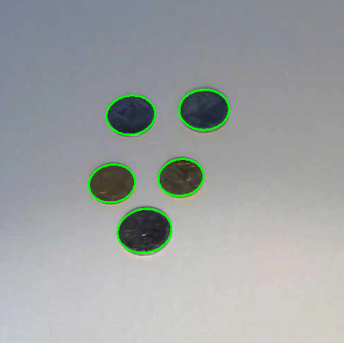
And finally, this is the result in the end of all steps described above:
The final image with the contours detected
The complete source-code:
import numpy as np
import cv2
def run_main():
cap = cv2.VideoCapture(0)
cap.set(cv2.cv.CV_CAP_PROP_FRAME_WIDTH, 1280)
cap.set(cv2.cv.CV_CAP_PROP_FRAME_HEIGHT, 720)
while(True):
ret, frame = cap.read()
roi = frame[0:500, 0:500]
gray = cv2.cvtColor(roi, cv2.COLOR_BGR2GRAY)
gray_blur = cv2.GaussianBlur(gray, (15, 15), 0)
thresh = cv2.adaptiveThreshold(gray_blur, 255, cv2.ADAPTIVE_THRESH_GAUSSIAN_C,
cv2.THRESH_BINARY_INV, 11, 1)
kernel = np.ones((3, 3), np.uint8)
closing = cv2.morphologyEx(thresh, cv2.MORPH_CLOSE, kernel, iterations=4)
cont_img = closing.copy()
contours, hierarchy = cv2.findContours(cont_img, cv2.RETR_EXTERNAL,
cv2.CHAIN_APPROX_SIMPLE)
for cnt in contours:
    area = cv2.contourArea(cnt)
    if area < 2000 or area > 4000:
        continue

    if len(cnt) < 5:
        continue

    ellipse = cv2.fitEllipse(cnt)
    cv2.ellipse(roi, ellipse, (0,255,0), 2)
cv2.imshow("Morphological Closing", closing)
cv2.imshow("Adaptive Thresholding", thresh)
cv2.imshow('Contours', roi)
if cv2.waitKey(1) & 0xFF == ord('q'):
break
cap.release()
cv2.destroyAllWindows()
if __name__ == "__main__":
run_main()
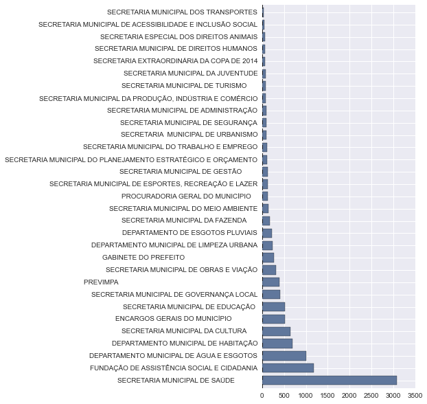
Há poucos dias, a prefeitura de Porto Alegre liberou os datasets com os dados de despesas de custeio de vários órgãos municipais (Secretaria Municipal de Saúde, Secretaria Municipal de Cultura, Gabinete do Prefeito, etc.). O plot abaixo mostra a quantidade de empenhos para cada órgão municipal:
Plot – Qtd Empenhos vs Órgãos
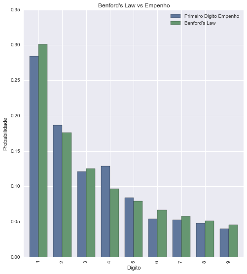
Uma das maneiras utilizadas geralmente para verificar fraudes é o uso da Lei de Benford[1][2][3], que fala sobre a distribuição das frequências de dígitos em vários datasets da vida real, incluindo valores de ações, número de populações, tamanhos de rios, etc.
Ao correlacionar a distribuição de números dos primeiros digitos dos valores de empenhos dos dados de Despesas de Custeio do 2º bimestre de 2014 com a distribuição da Lei de Benford, a correlação ficou muito clara:
Lei de Benford vs Despesas de Custeio (Empenho)
Segue aí mais um exemplo de correlação da Lei de Benford. Um sistema legal para ser construído seria um monitor de despesas que verificasse a correlação da Lei de Benford automaticamente e alertasse a cada anomalia encontrada.
So, in mathematics, we have the concept of universality in which we have laws like the law of large numbers, the Benford’s law (that I cited a lot in previous posts), the central limit theorem, and many other laws that act like laws of physics for the world of mathematics. These laws are not our inventions, I mean, the concepts are our inventions but the laws per se are universal, they are true no matter where you are on the earth or if you live far away in the universe. And that is why Frank Drake, one of the founders of SETI and also one of the pioneers in the search for extraterrestrial intelligence came with this brilliant idea of using prime numbers (another example of universality) to communicate with distant worlds. The idea that Frank Drake had was the use of prime numbers to hide (not actually hide, but to make self-evident, you’ll understand later) the dimension of a transmitted image in the image size itself.
So, imagine you are receiving a message that is a sequence of dashes and dots like “—.-.—.-.——–…-.—” that repeats after a short pause and then again and again. Let’s suppose that this message has a size of 1679 symbols. So you begin analyzing the number, which is, in fact, a semiprime number (the same used in cryptography, a number that is a product of two prime numbers) that can be factored in prime factors as 23*73=1679, and this is the only way to factor it in prime factors (actually all numbers have only a single set of prime factors that are unique, see Fundamental theorem of arithmetic). So, since there are only two prime factors, you will try to reshape the signal in a 2D image and this image can have the dimension of 23×73 or 73×23, when you arrange the image in one of these dimensions you’ll see that the image makes sense and the other will be just a random and strange sequence. By using prime numbers (or semiprimes) you just used the total image size to define the only two possible ways of arranging the image dimension.
Arecibo Observatory
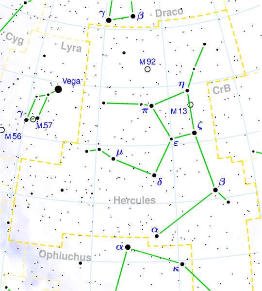
This idea was actually used in reality in 1974 by the Arecibo radio telescope when a message was broadcast in frequency modulation (FM) aiming the M13 globular star cluster at 25.000 light-years away:
M13 Globular Star Cluster
This message had the size (surprise) of 1679 binary digits and carried a lot of information about your world like a graphical representation of a human, numbers from 1 to 10, a graphical representation of the Arecibo radio telescope, etc.
The message decoded as 23 rows and 73 columns are this:
Arecibo Message Shifted (Source: Wikipedia)
As you can see, the message looks a lot nonsensical, but when it is decoded as an image with 73 rows and 23 columns, it will show its real significance:
Arecibo Message with the correct dimension (Source: Wikipedia)
This website uses cookies to improve your experience. We'll assume you're ok with this, but you can opt-out if you wish. Cookie settingsACCEPT
Privacy & Cookies Policy
Privacy Overview
This website uses cookies to improve your experience while you navigate through the website. Out of these cookies, the cookies that are categorized as necessary are stored on your browser as they are essential for the working of basic functionalities of the website. We also use third-party cookies that help us analyze and understand how you use this website. These cookies will be stored in your browser only with your consent. You also have the option to opt-out of these cookies. But opting out of some of these cookies may have an effect on your browsing experience.
Necessary cookies are absolutely essential for the website to function properly. This category only includes cookies that ensures basic functionalities and security features of the website. These cookies do not store any personal information.
Any cookies that may not be particularly necessary for the website to function and is used specifically to collect user personal data via analytics, ads, other embedded contents are termed as non-necessary cookies. It is mandatory to procure user consent prior to running these cookies on your website.