The new issue of SIGEVOlution is public available !
In this issue, you’ll found an interview with Hans-Paul Schwefel by my fellow countryman, Marcelo de Brito (or Genetic Argonaut). Congratulations to the board !
by Christian S. Perone
The new issue of SIGEVOlution is public available !
In this issue, you’ll found an interview with Hans-Paul Schwefel by my fellow countryman, Marcelo de Brito (or Genetic Argonaut). Congratulations to the board !
Some time ago I’d done a post about acessing the MODIS near-real time satellite images using Python and the data public available at NASA MODIS, if you are interested in those images, take a look in the post here.
I’ve created now a Python package called pyearthquake to automatic retrieve any MODIS subset image from the NASA Rapid Response System in a easy way, just by using the subset, satellite and resolution parameters. The package has a module to get real-time USGS Earthquake data from the USGS website and automatically parse it for you, as well functions to retrieve shakemaps and other products from the USGS.
Let’s start talking about the public available catalogs with real-time Earthquake data from the USGS site (they are in CSV formats, there are others in XML and KMZ formats if you’re interested too, but I focused in the CSV format files to create the Python modules:
Note from USGS site: files are not inclusive (the past day file does not include past hour events, for example).
M1+ Earthquakes (past hour) – M1+PAST_HOUR
This is the worldwide catalog with earthquake data from the past hour;
M1+ Earthquakes (past day) – M1+PAST_DAY
This is the worldwide catalog with earthquake data from the past day;
M1+ Earthquakes (past 7 days) – M1+PAST_7DAY
This is the worldwide catalog with earthquake data from the past 7 days;
To get and process data from these catalogs, you can use the pyearthquake package I created, let’s install it first:
easy_install pyearthquake
This command will use the easy_install to automatic install the package from the PyPI respository, it will automatically resolve the requirements too, but if you face some problem, here is the explicit requirements: matplotlib >= 0.99.0, numpy >= 1.3.0, PIL >= 1.1.6 and basemap >= 0.99.4. The basemap package is map toolkit for matplotlib.
Let’s now, for example, get the catalog for the past hour earthquake data, we can do it by using the Python interpreter prompt, like this:
>>> catalog = usgs.retrieve_catalog("M1+PAST_HOUR")
>>> catalog
<pyearthquake.usgs.USGSCatalog instance at 0x00BD0FD0>
All catalogs available are: M1+PAST_HOUR, M1+PAST_DAY and M1+PAST_7DAY. But if you type a wrong catalog name, it will show you the name of all available.
You can now work with the “catalog” object to explore the data retrieved from the USGS site:
>>> list(catalog)
[{'Src': 'ci', 'Region': 'Central California', 'Lon': '-118.2063', 'Datetime': 'Saturday, January 16, 2010 17:12:20 UTC', 'Depth':
 '6.00', 'Version': '1', 'Lat': '36.2061', 'Eqid': '10530221', 'Magnitude': '1.9', 'NST': '27'}, {'Src': 'ak', 'Region': 'Southern
 Alaska', 'Lon': '-150.0829', 'Datetime': 'Saturday, January 16, 2010 16:47:05 UTC', 'Depth': '34.90', 'Version': '1', 'Lat': '61.
4521', 'Eqid': '10029267', 'Magnitude': '2.3', 'NST': '27'}]
>>> for row in catalog:
...    print row["Magnitude"], row["Depth"], row["Datetime"], row["Depth"], row["Region"]
...
1.9 6.00 Saturday, January 16, 2010 17:12:20 UTC 6.00 Central California
2.3 34.90 Saturday, January 16, 2010 16:47:05 UTC 34.90 Southern Alaska
As you can see, the “catalog” is an interable object where you can get all data from the earthquakes, like the Magnitude, Latitude, Longitude, Depth, Date, Region Name, etc…
Let’s now get the past 7 days earthquake data:
>>> catalog = usgs.retrieve_catalog("M1+PAST_7DAY")
>>> len(catalog)
1142
In the past 7 days, there was 1.142 Magnitude 1+ earthquakes on earth, if we want to find the event for the last Haiti tragedy, we can filter the Magnitude of the catalog by 6.0 for example:
>>> magnitude6 = [event for event in catalog if float(event["Magnitude"]) >= 6.0]
>>> len(magnitude6)
3
>>> for row in magnitude6: ... print row["Eqid"], row["Magnitude"], row["Depth"], row["Datetime"], row["Depth"], row["Region"] ... 2010rla9 6.0 32.40 Thursday, January 14, 2010 14:03:40 UTC 32.40 south of the Mariana Islands 2010rja6 7.0 13.00 Tuesday, January 12, 2010 21:53:10 UTC 13.00 Haiti region 71338066 6.5 29.30 Sunday, January 10, 2010 00:27:39 UTC 29.30 offshore Northern California
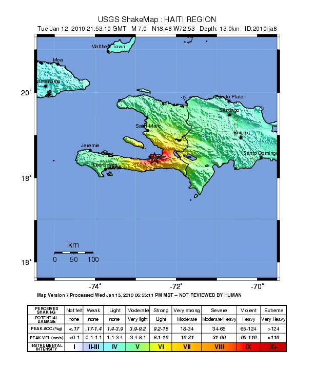
As we can see, the Earthquake ID “2010rja6” was the ID used by USGS to identify the 7.0 magnitude Haiti earthquake of the 12 January which has devastated the region and the unfortunate people of Haiti.
USGS also provides a Shakemaps, which are automatic computer generated maps with the potential damage in the region of the earthquake, to get it, let’s use the pyearthquake package:
>>> haiti_eq = magnitude6[1]
>>> usgs.retrieve_shakemap(haiti_eq, "INSTUMENTAL_INTENSITY")
 The second argument of the function is the shakemap type, there are other products you can get from USGS too, like the Media Maps, Peak Ground Acceleration. These maps are available in the package as: INSTRUMENTAL_INTENSITY, BARE, DECORATED, UNCERTAINTY and PEAK_GROUND_ACC.
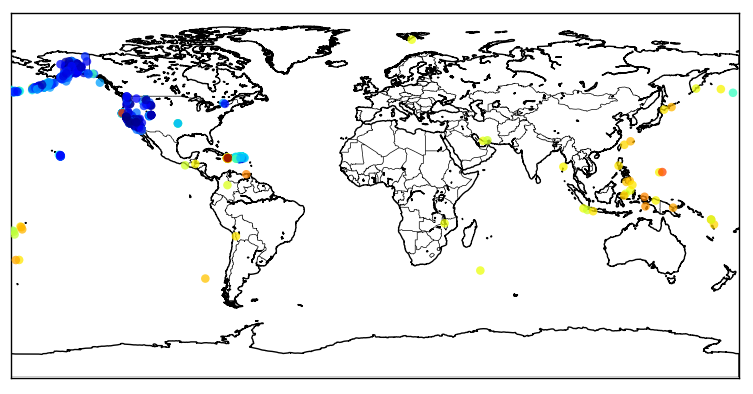
The packas has functions to plot maps of the earthquakes (using Matplotlib), see how to plot a map of the earthquakes from the past 7 days:
>>> usgs.plot_events(catalog)
<mpl_toolkits.basemap.Basemap object at 0x01E6BDB0>
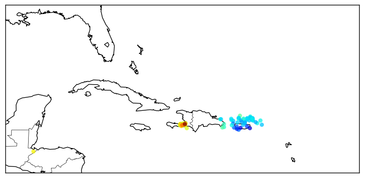
 Now a zoom in the Haiti region:
 The color of the points are relative to their magnitudes, I’m using here the JET (the yellow/red points are earthquakes with higher magnitudes) color map from Matplotlib, see in this link to use more color maps.
Let’s talk now about the “modis” module of the pyearthquake module. This module can be used to get the most recent or archived images (up to 250m resolution) from MODIS Aqua/Terra satellites. First of all, you must know what subset you want to retrieve from MODIS website, the subsets are available here in NASA site. To plot the Haiti region I’ll use the subset named “GreaterAntilles” which covers the Haiti region. To get the satellite images from today date, we can do like this:
>>> from pyearthquake import modis
>>> import datetime
>>> now = datetime.datetime.now()
>>> bmap = modis.get_modis_subset(now,
...                               "GreaterAntilles",
...                               satellite_name="terra",
...                               resolution="250m")
This command will get the composite image of the subset “GreaterAntilles” taken today from the “terra” satellite with a resolution of 250m (in fact, this will take a while, since I’m using a higher resolution here, the maximum is 250m). And here is the result:
And here is after a zoom into the Haiti region near of Port-au-Prince:
This is the interesting part about MODIS, this photo, is from TODAY.
Now, let’s merge together the information about the earthquakes from the USGS data and the recent images from the Haiti:
import datetime
from pyearthquake import usgs
from pyearthquake import modis

catalog = usgs.retrieve_catalog("M1+PAST_7DAY")

now = datetime.datetime.now()
bmap = modis.get_modis_subset(now,
                              "GreaterAntilles",
                              satellite_name="terra",
                              resolution="250m",
                              show=False)
usgs.plot_events(catalog, bmap)
And here is the result of the past 7 days earthquakes plot over the today MODIS image from satellite Terra:
That’s all =) you can use the package to plot earthquakes over other regions of world too, just select another subset from the MODIS Rapid Response System site.
– Christian S. Perone
All images and data shown here are from MODIS Response System or U.S. Geological Survey.
Here is the video of Pyevolve (the development version) optimizing a 100 cities TSP problem. I’ve used the Edge Recombination and the simple Swap Mutation method:
The video is a composition the of image outputs at every 100th generation and only when the score has changed when compared to the previous generation. I’ll release the source together with the new 0.6 release, planned to this month (December) and no later than January.
Best wishes and if I can’t post again until the next year, merry christmas and happy new year !!!
– Christian S. Perone

Hello folks, I always post about Python and EvoComp (Pyevolve), but this time it’s about C, LLVM, search algorithms and data structures. This post describes the efforts to implement an idea: to JIT (verb) algorithms and the data structures used by them, together.
Here is a short intro to AVL Trees from Wikipedia:
In computer science, an AVL tree is a self-balancing binary search tree, and it is the first such data structure to be invented. In an AVL tree, the heights of the two child subtrees of any node differ by at most one; therefore, it is also said to be height-balanced. Lookup, insertion, and deletion all take O(log n) time in both the average and worst cases, where n is the number of nodes in the tree prior to the operation. Insertions and deletions may require the tree to be rebalanced by one or more tree rotations.
When we have a data structure and algorithms to handle (insert, remove and lookup) that structure, the native code of our algorithm is usually full of overhead; for example, in an AVL Tree (Balanced Binary Tree), the overhead appear in: checking if we really have a left or right node while traversing the nodes for lookups, accessing nodes inside nodes, etc. This overhead creates unnecessary assembly operations which in turn, creates native code overhead, even when the compiler optimize it. This overhead directly impacts on the performance of our algorithm (this traditional approach, of course, give us a very flexible structure and the complexity (not Big-O) is easy to handle, but we pay for it: performance loss).
I’m proud to announce that Pyevolve is featuring on the last issue of SIGEVOlution (Volume 4, Issue 1), a newsletter from the ACM Special Interest Group on Evolutionary Computation. I would like to thank the newsletter editor Pier Luca Lanzi and the board for the corrections in the article and for the well done reformatted version of the paper.
Pyevolve is currently in version 0.5, in a few months I’ll be releasing the new 0.6 release with the new major features that are currently implemented in the development version only (you can check it at the subversion repository in sourceforge.net).
I hope you enjoy the article !
Yours,
– Christian S. Perone
So I did a comparative of Pyevolve GP/GA core in different Python interpreters. I’ve used my Pentium Core 2 Duo (E4500 @ 2.20GHz, 1GB RAM), using Ubuntu 9.04 and Windows XP SP3 just for IronPython 2.6.1 (IronPython doesn’t run with Mono, so I used the win xp with .net 2.0).
The interpreters used were:
I tried using 2009Q3 (the currently main trunk), but I think it’s unstable yet, cause it was more slow than 2009Q2, so I used 2009Q2; I compiled it with GCC 4.3.3 just using the default configure parameters (./configure).
I used the default CPython package of Ubuntu 9.04.
I used the default CPython package of Ubuntu 9.04 too, the python2.5 package.
I used the last svn version of the repository, the release 68612. My Pentium Core 2 Duo had only 1GB of RAM, and the PyPy translation process eats more RAM than Java (sorry for the joke), so I used a notebook with 3GB of RAM to create the pypy-c, what took 1 hour (I used –opt=3) and a beautiful ascii Mandelbrot fractal !
I used the default installer from the Jython project site. I used the Sun JRE 1.6.0_16.
I’ve used the 2.6 RC1 available at IronPython project site with MS .NET 2.0.
To test the GA core I’ve used this source-code (a simple sphere function):
from pyevolve import G1DList
from pyevolve import Mutators, Initializators
from pyevolve import GSimpleGA, Consts

# This is the Sphere Function
def sphere(xlist):
   total = 0
   for i in xlist:
      total += i**2
   return total

def run_main():
   genome = G1DList.G1DList(140)
   genome.setParams(rangemin=-5.12, rangemax=5.13)
   genome.initializator.set(Initializators.G1DListInitializatorReal)
   genome.mutator.set(Mutators.G1DListMutatorRealGaussian)
   genome.evaluator.set(sphere)

   ga = GSimpleGA.GSimpleGA(genome, seed=666)
   ga.setMinimax(Consts.minimaxType["minimize"])
   ga.setGenerations(1500)
   ga.setMutationRate(0.01)
   ga.evolve(freq_stats=500)

   best = ga.bestIndividual()

if __name__ == "__main__":
   run_main()
And to test the GP core, I’ve used this source-code (a simple symbolic regression):
from pyevolve import GTree
from pyevolve import Mutators
from pyevolve import GSimpleGA, Consts, Util
import math

rmse_accum = Util.ErrorAccumulator()

def gp_add(a, b): return a+b
def gp_sub(a, b): return a-b
def gp_mul(a, b): return a*b
def gp_sqrt(a):   return math.sqrt(abs(a))

def eval_func(chromosome):
   global rmse_accum
   rmse_accum.reset()
   code_comp = chromosome.getCompiledCode()

   for a in xrange(0, 10):
      for b in xrange(0, 10):
         evaluated     = eval(code_comp)
         target        = math.sqrt((a*a)+(b*b))
         rmse_accum   += (target, evaluated)
   return rmse_accum.getRMSE()

def main_run():
   genome = GTree.GTreeGP()
   genome.setParams(max_depth=4, method="ramped")
   genome.evaluator += eval_func
   genome.mutator.set(Mutators.GTreeGPMutatorSubtree)

   ga = GSimpleGA.GSimpleGA(genome, seed=666)
   ga.setParams(gp_terminals       = ['a', 'b'],
                gp_function_prefix = "gp")

   ga.setMinimax(Consts.minimaxType["minimize"])
   ga.setGenerations(40)
   ga.setCrossoverRate(1.0)
   ga.setMutationRate(0.08)
   ga.setPopulationSize(800)

   ga(freq_stats=10)
   best = ga.bestIndividual()

if __name__ == "__main__":
   main_run()
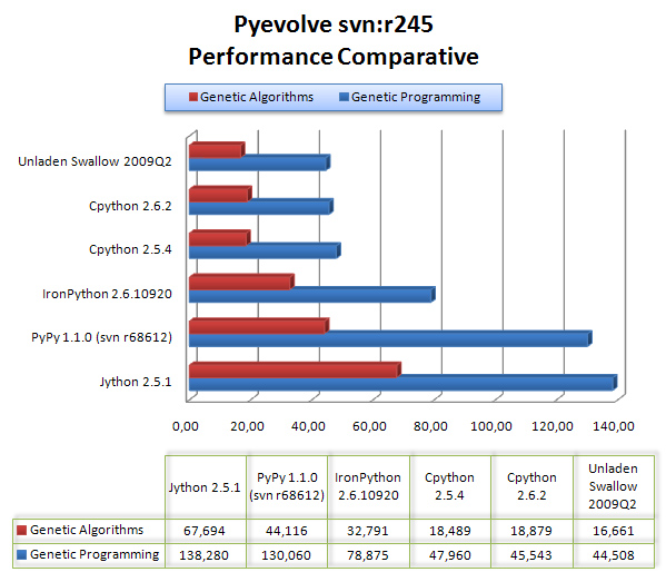
UPDATE 19/08: the x-axis is measured in “seconds“, and the y-axis is the python flavor;
The results are are described in the graph below:
 As we can see, Unladen Swallow 2009Q2 did a little better performance than CPython 2.6.2, but Jython and PyPy (experimental) were left behind in that scenario, even behind IronPython 2.6.1.
As we know, Genetic Programming usually requires intensive processing power for the fitness functions and tree manipulations (in crossover operations), and this fact can be a huge problem when using a pure Python approach like Pyevolve. So, to overcome this situation, I’ve used the Python multiprocessing features to implement a parallel fitness evaluation approach in Pyevolve and I was surprised by the super linear speedup I got for a cpu bound fitness function used to do the symbolic regression of the Pythagoras theorem: . I’ve used the same seed for the GP, so it has consumed nearly the same cpu resources for both test categories. Here are the results I obtained:
The first fitness landscape I’ve used had 2.500 points and the later had a fitness landscape of 6.400 points, here is the source code I’ve used (you just need to turn on the multiprocessing option using the setMultiProcessing method, so Pyevolve will use multiprocessing when you have more than one single core, you can enable the logging feature to check what’s going on behind the scenes):
from pyevolve import *
import math

rmse_accum = Util.ErrorAccumulator()

def gp_add(a, b): return a+b
def gp_sub(a, b): return a-b
def gp_mul(a, b): return a*b
def gp_sqrt(a):   return math.sqrt(abs(a))

def eval_func(chromosome):
   global rmse_accum
   rmse_accum.reset()
   code_comp = chromosome.getCompiledCode()

   for a in xrange(0, 80):
      for b in xrange(0, 80):
         evaluated     = eval(code_comp)
         target        = math.sqrt((a*a)+(b*b))
         rmse_accum   += (target, evaluated)
   return rmse_accum.getRMSE()

def main_run():
   genome = GTree.GTreeGP()
   genome.setParams(max_depth=4, method="ramped")
   genome.evaluator += eval_func
   genome.mutator.set(Mutators.GTreeGPMutatorSubtree)

   ga = GSimpleGA.GSimpleGA(genome, seed=666)
   ga.setParams(gp_terminals       = ['a', 'b'],
                gp_function_prefix = "gp")

   ga.setMinimax(Consts.minimaxType["minimize"])
   ga.setGenerations(20)
   ga.setCrossoverRate(1.0)
   ga.setMutationRate(0.08)
   ga.setPopulationSize(800)
   ga.setMultiProcessing(True)

   ga(freq_stats=5)
   best = ga.bestIndividual()

if __name__ == "__main__":
   main_run()
As you can see, the population size was 800 individuals with a 8% mutation rate and a 100% crossover rate for a simple 20 generations evolution. Of course you don’t need so many points in the fitness landscape, I’ve used 2.500+ points to create a cpu intensive fitness function, otherwise, the speedup can be less than 1.0 due the communication overhead between the processes. For the first case (2.500 points fitness landscape) I’ve got a 3.33x speedup and for the last case (6.400 points fitness landscape) I’ve got a 3.28x speedup. The tests were executed in a 2 cores pc (Intel Core 2 Duo).
UPDATE 05/10: there is an article in the Physorg too.
Sometimes we face new applications for EC, but for this I was not expecting, from Eurekalert:
WASHINGTON, Oct. 5 — Criminals are having a harder time hiding their faces, thanks to new software that helps witnesses recreate and recognize suspects using principles borrowed from the fields of optics and genetics.
(…)
His software generates its own faces that progressively evolve to match the witness’ memories. The witness starts with a general description such as “I remember a young white male with dark hair.” Nine different computer-generated faces that roughly fit the description are generated, and the witness identifies the best and worst matches. The software uses the best fit as a template to automatically generate nine new faces with slightly tweaked features, based on what it learned from the rejected faces.
“Over a number of generations, the computer can learn what face you’re looking for,” says Solomon.
Read the full article here.