Hi all ! This post is to celebrate 10 years of blogging with an average of 1 post per month. It was a quite cool adventure !
Here is the full table of contents for those interested:
by Christian S. Perone
Hi all ! This post is to celebrate 10 years of blogging with an average of 1 post per month. It was a quite cool adventure !
Here is the full table of contents for those interested:
It is frustrating to learn about principles such as maximum likelihood estimation (MLE), maximum a posteriori (MAP) and Bayesian inference in general. The main reason behind this difficulty, in my opinion, is that many tutorials assume previous knowledge, use implicit or inconsistent notation, or are even addressing a completely different concept, thus overloading these principles.
Those aforementioned issues make it very confusing for newcomers to understand these concepts, and I’m often confronted by people who were unfortunately misled by many tutorials. For that reason, I decided to write a sane introduction to these concepts and elaborate more on their relationships and hidden interactions while trying to explain every step of formulations. I hope to bring something new to help people understand these principles.
The maximum likelihood estimation is a method or principle used to estimate the parameter or parameters of a model given observation or observations. Maximum likelihood estimation is also abbreviated as MLE, and it is also known as the method of maximum likelihood. From this name, you probably already understood that this principle works by maximizing the likelihood, therefore, the key to understand the maximum likelihood estimation is to first understand what is a likelihood and why someone would want to maximize it in order to estimate model parameters.
Let’s start with the definition of the likelihood function for continuous case:
$$\mathcal{L}(\theta | x) = p_{\theta}(x)$$
The left term means “the likelihood of the parameters \(\theta\), given data \(x\)”. Now, what does that mean ? It means that in the continuous case, the likelihood of the model \(p_{\theta}(x)\) with the parametrization \(\theta\) and data \(x\) is the probability density function (pdf) of the model with that particular parametrization.
Although this is the most used likelihood representation, you should pay attention that the notation \(\mathcal{L}(\cdot | \cdot)\) in this case doesn’t mean the same as the conditional notation, so be careful with this overload, because it is always implicitly stated and it is also often a source of confusion. Another representation of the likelihood that is often used is \(\mathcal{L}(x; \theta)\), which is better in the sense that it makes it clear that it’s not a conditional, however, it makes it look like the likelihood is a function of the data and not of the parameters.
The model \(p_{\theta}(x)\) can be any distribution, and to make things concrete, let’s say that we are assuming that the data generating distribution is an univariate Gaussian distribution, which we define below:
$$
\begin{align}
p(x) & \sim \mathcal{N}(\mu, \sigma^2) \\
p(x; \mu, \sigma^2) & \sim \frac{1}{\sqrt{2\pi\sigma^2}} \exp{ \bigg[-\frac{1}{2}\bigg( \frac{x-\mu}{\sigma}\bigg)^2 \bigg] }
\end{align}
$$
If you plot this probability density function with different parametrizations, you’ll get something like the plots below, where the red distribution is the standard Gaussian \(p(x) \sim \mathcal{N}(0, 1.0)\):
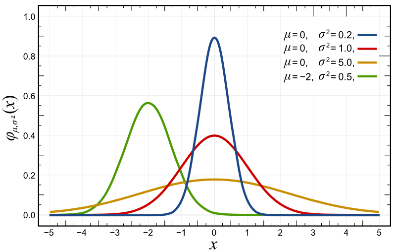
As you can see in the probability density function (pdf) plot above, the likelihood of \(x\) at variously given realizations are showed in the y-axis. Another source of confusion here is that usually, people take this as a probability, because they usually see these plots of normals and the likelihood is always below 1, however, the probability density function doesn’t give you probabilities but densities. The constraint on the pdf is that it must integrate to one:
$$\int_{-\infty}^{+\infty} f(x)dx = 1$$
So, it is completely normal to have densities larger than 1 in many points for many different distributions. Take for example the pdf for the Beta distribution below:
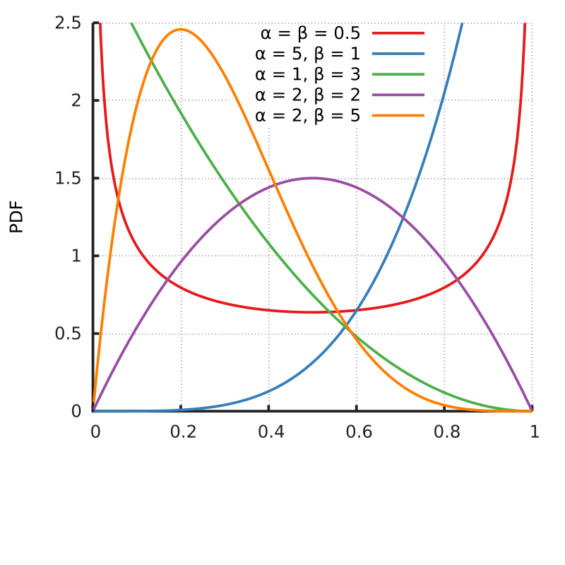
As you can see, the pdf shows densities above one in many parametrizations of the distribution, while still integrating into 1 and following the second axiom of probability: the unit measure.
So, returning to our original principle of maximum likelihood estimation, what we want is to maximize the likelihood \(\mathcal{L}(\theta | x)\) for our observed data. What this means in practical terms is that we want to find the parameters \(\theta\) of our model where the likelihood that this model generated our data is maximized, we want to find which parameters of this model are most plausible to have generated this observed data, or what are the parameters that make this sample most probable ?
For the case of our univariate Gaussian model, what we want is to find the parameters \(\mu\) and \(\sigma^2\), which for convenient notation we collapse into a single parameter vector:
$$\theta = \begin{bmatrix}\mu \\ \sigma^2\end{bmatrix}$$
Because these are the statistics that completely define our univariate Gaussian model. So let’s formulate the problem of the maximum likelihood estimation:
$$
\begin{align}
\hat{\theta} &= \mathrm{arg}\max_\theta \mathcal{L}(\theta | x) \\
&= \mathrm{arg}\max_\theta p_{\theta}(x)
\end{align}
$$
This says that we want to obtain the maximum likelihood estimate \(\hat{\theta}\) that approximates \(p_{\theta}(x)\) to a underlying “true” distribution \(p_{\theta^*}(x)\) by maximizing the likelihood of the parameters \(\theta\) given data \(x\). You shouldn’t confuse a maximum likelihood estimate \(\hat{\theta}(x)\) which is a realization of the maximum likelihood estimator for the data \(x\), with the maximum likelihood estimator \(\hat{\theta}\), so pay attention to disambiguate it in your head.
However, we need to incorporate multiple observations in this formulation, and by adding multiple observations we end up with a complex joint distribution:
$$\hat{\theta} = \mathrm{arg}\max_\theta p_{\theta}(x_1, x_2, \ldots, x_n)$$
That needs to take into account the interactions between all observations. And here is where we make a strong assumption: we state that the observations are independent. Independent random variables mean that the following holds:
$$p_{\theta}(x_1, x_2, \ldots, x_n) = \prod_{i=1}^{n} p_{\theta}(x_i)$$
Which means that since \(x_1, x_2, \ldots, x_n\) don’t contain information about each other, we can write the joint probability as a product of their marginals.
Another assumption that is made, is that these random variables are identically distributed, which means that they came from the same generating distribution, which allows us to model it with the same distribution parametrization.
Given these two assumptions, which are also known as IID (independently and identically distributed), we can formulate our maximum likelihood estimation problem as:
$$\hat{\theta} = \mathrm{arg}\max_\theta \prod_{i=1}^{n} p_{\theta}(x_i)$$
Note that MLE doesn’t require you to make these assumptions, however, many problems will appear if you don’t to it, such as different distributions for each sample or having to deal with joint probabilities.
Given that in many cases these densities that we multiply can be very small, multiplying one by the other in the product that we have above we can end up with very small values. Here is where the logarithm function makes its way to the likelihood. The log function is a strictly monotonically increasing function, that preserves the location of the extrema and has a very nice property:
$$\log ab = \log a + \log b $$
Where the logarithm of a product is the sum of the logarithms, which is very convenient for us, so we’ll apply the logarithm to the likelihood to maximize what is called the log-likelihood:
$$
\begin{align}
\hat{\theta} &= \mathrm{arg}\max_\theta \prod_{i=1}^{n} p_{\theta}(x_i) \\
&= \mathrm{arg}\max_\theta \sum_{i=1}^{n} \log p_{\theta}(x_i) \\
\end{align}
$$
As you can see, we went from a product to a summation, which is much more convenient. Another reason for the application of the logarithm is that we often take the derivative and solve it for the parameters, therefore is much easier to work with a summation than a multiplication.
We can also conveniently average the log-likelihood (given that we’re just including a multiplication by a constant):
$$
\begin{align}
\hat{\theta} &= \mathrm{arg}\max_\theta \sum_{i=1}^{n} \log p_{\theta}(x_i) \\
&= \mathrm{arg}\max_\theta \frac{1}{n} \sum_{i=1}^{n} \log p_{\theta}(x_i) \\
\end{align}
$$
This is also convenient because it will take out the dependency on the number of observations. We also know, that through the law of large numbers, the following holds as \(n\to\infty\):
$$
\frac{1}{n} \sum_{i=1}^{n} \log \, p_{\theta}(x_i) \approx \mathbb{E}_{x \sim p_{\theta^*}(x)}\left[\log \, p_{\theta}(x) \right]
$$
As you can see, we’re approximating the expectation with the empirical expectation defined by our dataset \(\{x_i\}_{i=1}^{n}\). This is an important point and it is usually implictly assumed.
The weak law of large numbers can be bounded using a Chebyshev bound, and if you are interested in concentration inequalities, I’ve made an article about them here where I discuss the Chebyshev bound.
To finish our formulation, given that we usually minimize objectives, we can formulate the same maximum likelihood estimation as the minimization of the negative of the log-likelihood:
$$
\hat{\theta} = \mathrm{arg}\min_\theta -\mathbb{E}_{x \sim p_{\theta^*}(x)}\left[\log \, p_{\theta}(x) \right]
$$
Which is exactly the same thing with just the negation turn the maximization problem into a minimization problem.
It is well-known that maximizing the likelihood is the same as minimizing the Kullback-Leibler divergence, also known as the KL divergence. Which is very interesting because it links a measure from information theory with the maximum likelihood principle.
The KL divergence is defined as:
$$
\begin{equation}
D_{KL}( p || q)=\int p(x)\log\frac{p(x)}{q(x)} \ dx
\end{equation}
$$
There are many intuitions to understand the KL divergence, I personally like the perspective on the likelihood ratios, however, there are plenty of materials about it that you can easily find and it’s out of the scope of this introduction.
The KL divergence is basically the expectation of the log-likelihood ratio under the \(p(x)\) distribution. What we’re doing below is just rephrasing it by using some identities and properties of the expectation:
$$
\begin{align}
D_{KL}[p_{\theta^*}(x) \, \Vert \, p_\theta(x)] &= \mathbb{E}_{x \sim p_{\theta^*}(x)}\left[\log \frac{p_{\theta^*}(x)}{p_\theta(x)} \right] \\
\label{eq:logquotient}
&= \mathbb{E}_{x \sim p_{\theta^*}(x)}\left[\log \,p_{\theta^*}(x) – \log \, p_\theta(x) \right] \\
\label{eq:linearization}
&= \mathbb{E}_{x \sim p_{\theta^*}(x)} \underbrace{\left[\log \, p_{\theta^*}(x) \right]}_{\text{Entropy of } p_{\theta^*}(x)} – \underbrace{\mathbb{E}_{x \sim p_{\theta^*}(x)}\left[\log \, p_{\theta}(x) \right]}_{\text{Negative of log-likelihood}}
\end{align}
$$
In the formulation above, we’re first using the fact that the logarithm of a quotient is equal to the difference of the logs of the numerator and denominator (equation \(\ref{eq:logquotient}\)). After that we use the linearization of the expectation(equation \(\ref{eq:linearization}\)), which tells us that \(\mathbb{E}\left[X + Y\right] = \mathbb{E}\left[X\right]+\mathbb{E}\left[Y\right]\). In the end, we are left with two terms, the first one in the left is the entropy and the one in the right you can recognize as the negative of the log-likelihood that we saw earlier.
If we want to minimize the KL divergence for the \(\theta\), we can ignore the first term, since it doesn’t depend of \(\theta\) in any way, and in the end we have exactly the same maximum likelihood formulation that we saw before:
$$
\begin{eqnarray}
\require{cancel}
\theta^* &=& \mathrm{arg}\min_\theta \cancel{\mathbb{E}_{x \sim p_{\theta^*}(x)} \left[\log \, p_{\theta^*}(x) \right]} – \mathbb{E}_{x \sim p_{\theta^*}(x)}\left[\log \, p_{\theta}(x) \right]\\
&=& \mathrm{arg}\min_\theta -\mathbb{E}_{x \sim p_{\theta^*}(x)}\left[\log \, p_{\theta}(x) \right]
\end{eqnarray}
$$
A very common scenario in Machine Learning is supervised learning, where we have data points \(x_n\) and their labels \(y_n\) building up our dataset \( D = \{ (x_1, y_1), (x_2, y_2), \ldots, (x_n, y_n) \} \), where we’re interested in estimating the conditional probability of \(\textbf{y}\) given \(\textbf{x}\), or more precisely \( P_{\theta}(Y | X) \).
To extend the maximum likelihood principle to the conditional case, we just have to write it as:
$$
\hat{\theta} = \mathrm{arg}\min_\theta -\mathbb{E}_{x \sim p_{\theta^*}(y | x)}\left[\log \, p_{\theta}(y | x) \right]
$$
And then it can be easily generalized to formulate the linear regression:
$$
p_{\theta}(y | x) \sim \mathcal{N}(x^T \theta, \sigma^2) \\
\log p_{\theta}(y | x) = -n \log \sigma – \frac{n}{2} \log{2\pi} – \sum_{i=1}^{n}{\frac{\| x_i^T \theta – y_i \|}{2\sigma^2}}
$$
In that case, you can see that we end up with a sum of squared errors that will have the same location of the optimum of the mean squared error (MSE). So you can see that minimizing the MSE is equivalent of maximizing the likelihood for a Gaussian model.
The maximum likelihood estimation has very interesting properties but it gives us only point estimates, and this means that we cannot reason on the distribution of these estimates. In contrast, Bayesian inference can give us a full distribution over parameters, and therefore will allow us to reason about the posterior distribution.
I’ll write more about Bayesian inference and sampling methods such as the ones from the Markov Chain Monte Carlo (MCMC) family, but I’ll leave this for another article, right now I’ll continue showing the relationship of the maximum likelihood estimator with the maximum a posteriori (MAP) estimator.
Although the maximum a posteriori, also known as MAP, also provides us with a point estimate, it is a Bayesian concept that incorporates a prior over the parameters. We’ll also see that the MAP has a strong connection with the regularized MLE estimation.
We know from the Bayes rule that we can get the posterior from the product of the likelihood and the prior, normalized by the evidence:
$$
\begin{align}
p(\theta \vert x) &= \frac{p_{\theta}(x) p(\theta)}{p(x)} \\
\label{eq:proport}
&\propto p_{\theta}(x) p(\theta)
\end{align}
$$
In the equation \(\ref{eq:proport}\), since we’re worried about optimization, we cancel the normalizing evidence \(p(x)\) and stay with a proportional posterior, which is very convenient because the marginalization of \(p(x)\) involves integration and is intractable for many cases.
$$
\begin{align}
\theta_{MAP} &= \mathop{\rm arg\,max}\limits_{\theta} p_{\theta}(x) p(\theta) \\
&= \mathop{\rm arg\,max}\limits_{\theta} \prod_{i=1}^{n} p_{\theta}(x_i) p(\theta) \\
&= \mathop{\rm arg\,max}\limits_{\theta} \sum_{i=1}^{n} \underbrace{\log p_{\theta}(x_i)}_{\text{Log likelihood}} \underbrace{p(\theta)}_{\text{Prior}}
\end{align}
$$
In this formulation above, we just followed the same steps as described earlier for the maximum likelihood estimator, we assume independence and an identical distributional setting, followed later by the logarithm application to switch from a product to a summation. As you can see in the final formulation, this is equivalent as the maximum likelihood estimation multiplied by the prior term.
We can also easily recover the exact maximum likelihood estimator by using a uniform prior \(p(\theta) \sim \textbf{U}(\cdot, \cdot)\). This means that every possible value of \(\theta\) will be equally weighted, meaning that it’s just a constant multiplication:
$$
\begin{align}
\theta_{MAP} &= \mathop{\rm arg\,max}\limits_{\theta} \sum_i \log p_{\theta}(x_i) p(\theta) \\
&= \mathop{\rm arg\,max}\limits_{\theta} \sum_i \log p_{\theta}(x_i) \, \text{constant} \\
&= \underbrace{\mathop{\rm arg\,max}\limits_{\theta} \sum_i \log p_{\theta}(x_i)}_{\text{Equivalent to maximum likelihood estimation (MLE)}} \\
\end{align}
$$
And there you are, the MAP with a uniform prior is equivalent to MLE. It is also easy to show that a Gaussian prior can recover the L2 regularized MLE. Which is quite interesting, given that it can provide insights and a new perspective on the regularization terms that we usually use.
I hope you liked this article ! The next one will be about Bayesian inference with posterior sampling, where we’ll show how we can reason about the posterior distribution and not only on point estimates as seen in MAP and MLE.
– Christian S. Perone
![]()
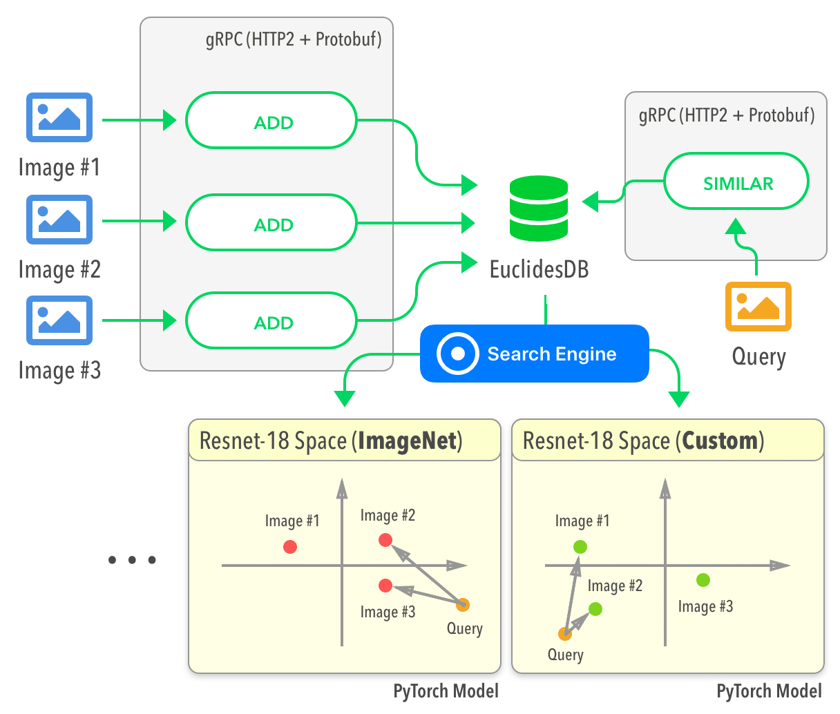
Past week I released the first public version of EuclidesDB. EuclidesDB is a multi-model machine learning feature database that is tightly coupled with PyTorch and provides a backend for including and querying data on the model feature space.
For more information, see the GitHub repository or the documentation.
Some features of EuclidesDB are listed below:
And here is a diagram of the overall architecture:
This last presidential election in Brazil was heavily marked by huge amounts of money being funneled to digital agencies and all kinds of targeting businesses that used Twitter, WhatsApp, and even SMS messages to propagate their content using their targeting strategies. Even before the elections, Cambridge Analytica was recorded mentioning their involvement in Brazil.
What makes Brazil so vulnerable for these micro-targeting companies, in my opinion, is the widespread ingenuity regarding digital platforms. An example of this ingenuity was the wide-spreading of applications that were allegedly developed to monitor politicians and give information about them, to help you decide your vote, bookmark politicians, etc. But in reality, it was more than clear that these applications were just capturing data (such as geolocation, personal opinions, demographics, etc) about their users with the intention to sell it later or use themselves for targeting. I even saw journalists and some very well-known people supporting these applications. Simply put, most of the time, when you don’t pay for a product (or application), you’re the product.
One very interesting work is the experiment done by Wu Youyou in 2014 where he showed that a simple regularized linear model was better or equal in accuracy to identify some personality traits using Facebook likes, this study used more than 80k participants data:
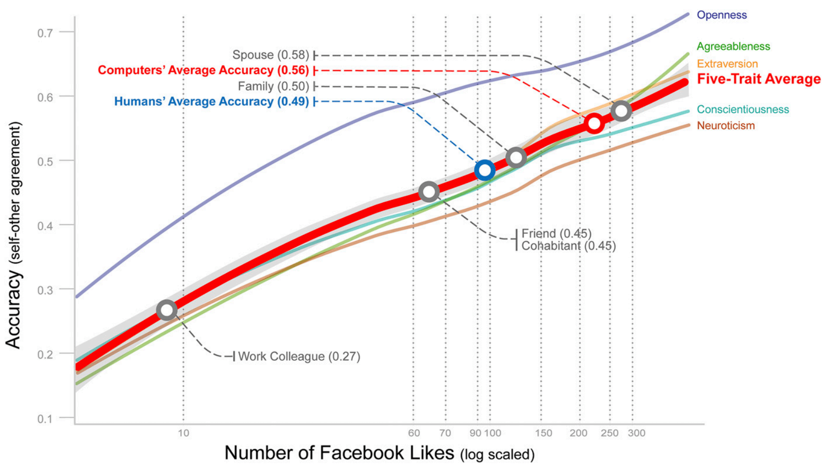
This graph above shows that with 70 likes from your Facebook, the linear model was more accurate than the evaluation of a friend of you and with more than 150 likes it can reach the accuracy of the evaluation of your family. Now you can understand why social data is so important for these companies to identify personality traits and content that you’re most susceptible.
In this year, one of the candidates didn’t participate much on the debates before the second round and used mostly digital platforms to reach voters, so Twitter became a very important medium that all candidates explored in some way. The idea of this post is to use a discrete event visualization technique called Time Maps which was extended to Twitter visualizations by Max C. Watson in his work “Time Maps: A Tool for Visualizing Many Discrete Events Across Multiple Timescales” (paper available here). It is unfortunate that not a lot of people use these visualizations because they are very interesting for the visualization of activity patterns in multiple time-scales on a single plot.
The main idea behind time maps is that you can visualize the time after and before the events for the entire discrete time events. This can be easily understood by looking at the visual explanations done by Max C. Watson.

As you can see in the right, the plot is pretty straightforward, it might take some time for you to realize what is the meaning of the x and y-axes, but once you grasp the concept, you’ll see that they are quite easy to interpret and how many patterns it can reveal on a single plot.
Time maps were an adaptation from the chaotic field where they were initially developed to study the timing of water drops.
One way to easily understand it is to look at these two series below and their respective time maps:

But before plotting the time maps, let’s explore some basic visualizations from the two candidates who got into the second round of the general elections last week.
I’ll focus only on the two candidates who got into the second round of the elections, their names are Jair Bolsonaro (president elected) and Fernando Haddad (not elected). These first plots will show the number of tweets per day during the year of 2018 and with some red marks indicating the first and second rounds of the elections:
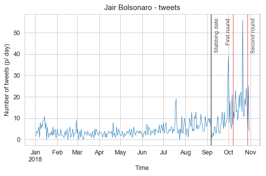
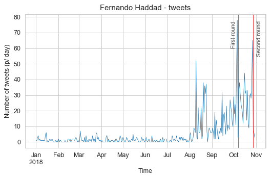 In these plots, we can see that Jair Bolsonaro was more active before the general elections and that for both candidates, the aggregated number of tweets per day always peaked before each election round, with Jair Bolsonaro peaks happening a little earlier than Fernando Haddad. I also marked with a black vertical line the day that Jair Bolsonaro was stabbed in the streets of Brazil, you can see a clear drop of activity with a slow recovery after it.
Let’s now see the time of day profile for each candidate to check the hours of the day that the candidates were quieter and more active:
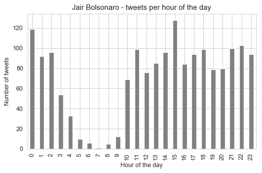
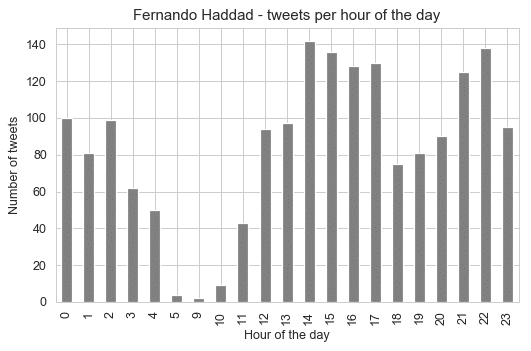 These profiles tell us very interesting information, that the candidates were most active between 3pm and 4pm, but for Jair Bolsonaro, it seems that the 3pm time of the day is really the time when he was most active by a significant margin. What is really interesting is that there is no tweet whatsoever between 6am and 8am for Fernando Haddad.
Let’s look now the distribution differences between 2017 and 2018 for each candidate:
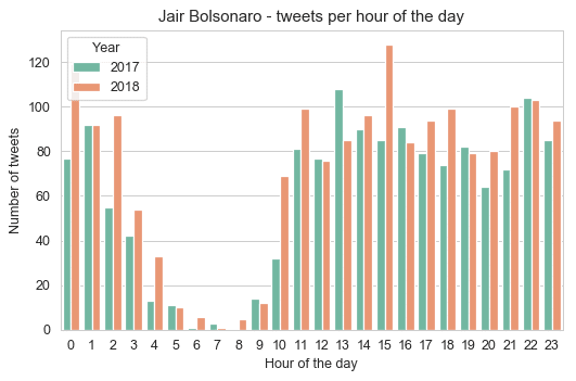
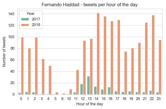 As we can see from these plots, Jair Bolsonaro was as active in 2017 as in 2018, while Fernando Haddad was not so much active in 2017 with a huge bump in a number of tweets in the year of 2018 (election year). Something that is interesting, is that the pattern from Jair Bolsonaro to tweet more at 1pm shifted to 3pm in 2018, while for Haddad it changed also from 1pm to 2pm. It can be hypothesized that before they were less involved and used to tweet after lunch, but during election year this routine changed (assuming that it’s not their staff who is managing the account for them), so there is not only more tweets but also a distributional shift in the hour of the day.
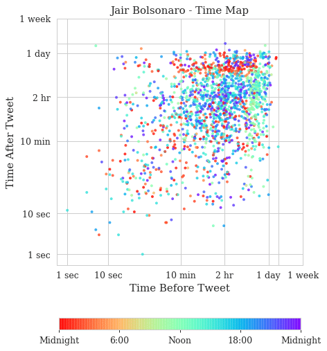
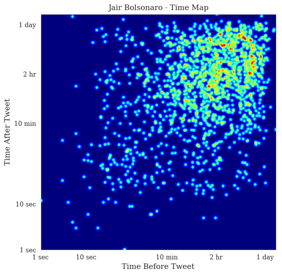
These are the time maps for Jair Bolsonaro. The first is the time map colored by the hour of the day and the second time map is a heat map to see the density of points in the time map.
And these are the time maps for Fernando Haddad:
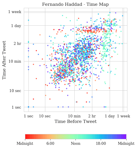
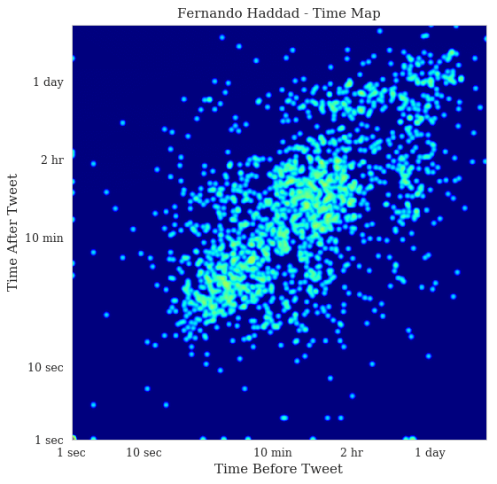 Now, these are very interesting time maps. You can clearly see in the Jair Bolsonaro time map that there are two stripes: vertical on the left and horizontal on the top that shows the first and last tweets of the day respectively. It’s a slow but steady activity of tweeting, with a concentration on the heat map on the 1-day bands. In Fernando Haddad, you can see that the stripes are still visible but much less concentrated. There are also two main blobs in the heat map of Fernando Haddad, one in the bottom left showing fast tweets that are probably from a specific event and then the blob on the top right showing the usual activity.
If you are interested in understanding more about these plots, please take a look on Max Watson blog article where he explains some interesting cases such as the tweets from the White House account.
If you are curious about how Twitter bots appear on time maps, here is an example where I plot the tweets from the CozinhaBot, that keeps posting some random recipes on twitter:
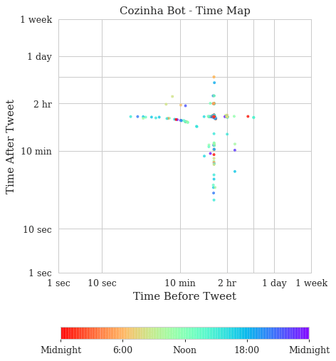
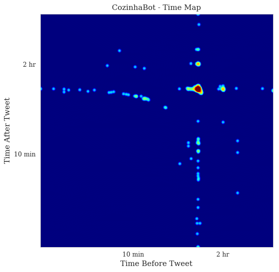
As you can see, the pattern is very regular, in the heat map we can see the huge density spot before the 2 hr ticks, which means that this bot has a very well known and regular pattern, as opposed to the human-produced patterns we saw before. These plots don’t have a small amount of dots because it has fewer tweets, but because they follow a very regular interval, this plot contains nearly the same amount of tweets we saw from the previous examples of the presidential candidates. This is very interesting because not only can be used to spot twitter bots but also to identify which tweets were posted out of the bot pattern.
I hope you liked !
– Christian S. Perone
* This post is in Portuguese. It’s a bayesian analysis of a Brazilian national exam. The main focus of the analysis is to understand the underlying factors impacting the participants performance on ENEM.
Este tutorial apresenta uma análise breve dos microdados do ENEM do Rio Grande do Sul do ano de 2017. O principal objetivo é entender os fatores que impactam na performance dos participantes do ENEM dado fatores como renda familiar e tipo de escola. Neste tutorial são apresentados dois modelos: regressão linear e regressão linear hierárquica.
I was experimenting with the digits distribution from a pre-trained (weights from the OpenAI repository) Transformer language model (LM) and I found a very interesting correlation between the Benford’s law and the digit distribution of the language model after conditioning it with some particular phrases.
Below is the correlation between the Benford’s law and the language model with conditioning on the phrase (shown in the figure):
![]()
Update 28 Feb 2019: I added a new blog post with a slide deck containing the presentation I did for PyData Montreal.
Today, at the PyTorch Developer Conference, the PyTorch team announced the plans and the release of the PyTorch 1.0 preview with many nice features such as a JIT for model graphs (with and without tracing) as well as the LibTorch, the PyTorch C++ API, one of the most important release announcement made today in my opinion.
Given the huge interest in understanding how this new API works, I decided to write this article showing an example of many opportunities that are now open after the release of the PyTorch C++ API. In this post, I’ll integrate PyTorch inference into native NodeJS using NodeJS C++ add-ons, just as an example of integration between different frameworks/languages that are now possible using the C++ API.
Below you can see the final result:
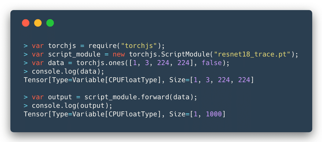
As you can see, the integration is seamless and I could use a traced ResNet as the computational graph model and feed any tensor to it to get the output predictions.
Simply put, the libtorch is a library version of the PyTorch. It contains the underlying foundation that is used by PyTorch, such as the ATen (the tensor library), which contains all the tensor operations and methods. Libtorch also contains the autograd, which is the component that adds the automatic differentiation to the ATen tensors.
A word of caution for those who are starting now is to be careful with the use of the tensors that can be created both from ATen and autograd, do not mix them, the ATen will return the plain tensors (when you create them using the at namespace) while the autograd functions (from the torch namespace) will return Variable, by adding its automatic differentiation mechanism.
For a more extensive tutorial on how PyTorch internals work, please take a look on my previous tutorial on the PyTorch internal architecture.
Libtorch can be downloaded from the Pytorch website and it is only available as a preview for a while. You can also find the documentation in this site, which is mostly a Doxygen rendered documentation. I found the library pretty stable, and it makes sense because it is actually exposing the stable foundations of PyTorch, however, there are some issues with headers and some minor problems concerning the library organization that you might find while starting working with it (that will hopefully be fixed soon).

For NodeJS, I’ll use the Native Abstractions library (nan) which is the most recommended library (actually is basically a header-only library) to create NodeJS C++ add-ons and the cmake-js, because libtorch already provide the cmake files that make our building process much easier. However, the focus here will be on the C++ code and not on the building process.
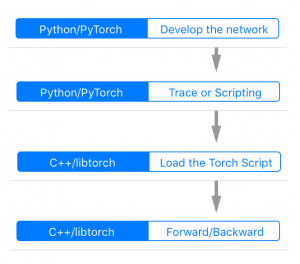
The flow for the development, tracing, serializing and loading the model can be seen in the figure on the left side.
It starts with the development process and tracing being done in PyTorch (Python domain) and then the loading and inference on the C++ domain (in our case in NodeJS add-on).
In NodeJS, to create an object as a first-class citizen of the JavaScript world, you need to inherit from the ObjectWrap class, which will be responsible for wrapping a C++ component.
#ifndef TENSOR_H
#define TENSOR_H

#include <nan.h>
#include <torch/torch.h>

namespace torchjs {

class Tensor : public Nan::ObjectWrap {
 public:
  static NAN_MODULE_INIT(Init);

  void setTensor(at::Tensor tensor) {
    this->mTensor = tensor;
  }

  torch::Tensor getTensor() {
    return this->mTensor;
  }

  static v8::Local<v8::Object> NewInstance();

 private:
  explicit Tensor();
  ~Tensor();

  static NAN_METHOD(New);
  static NAN_METHOD(toString);
  static Nan::Persistent<v8::Function> constructor;

 private:
  torch::Tensor mTensor;

};

}  // namespace torchjs

#endif
As you can see, most of the code for the definition of our Tensor class is just boilerplate. The key point here is that the torchjs::Tensor will wrap a torch::Tensor and we added two special public methods (setTensor and getTensor) to set and get this internal torch tensor.

I won’t show all the implementation details because most parts of it are NodeJS boilerplate code to construct the object, etc. I’ll focus on the parts that touch the libtorch API, like in the code below where we are creating a small textual representation of the tensor to show on JavaScript (toString method):
NAN_METHOD(Tensor::toString) {
  Tensor* obj = ObjectWrap::Unwrap<Tensor>(info.Holder());
  std::stringstream ss;

  at::IntList sizes = obj->mTensor.sizes();
  ss << "Tensor[Type=" << obj->mTensor.type() << ", ";
  ss << "Size=" << sizes << std::endl;

  info.GetReturnValue().Set(Nan::New(ss.str()).ToLocalChecked());
}
What we are doing in the code above, is just getting the internal tensor object from the wrapped object by unwrapping it. After that, we build a string representation with the tensor size (each dimension sizes) and its type (float, etc).
Let’s create now a wrapper code for the torch::ones function which is responsible for creating a tensor of any defined shape filled with constant 1’s.
NAN_METHOD(ones) {
  // Sanity checking of the arguments
  if (info.Length() < 2)
    return Nan::ThrowError(Nan::New("Wrong number of arguments").ToLocalChecked());

  if (!info[0]->IsArray() || !info[1]->IsBoolean())
    return Nan::ThrowError(Nan::New("Wrong argument types").ToLocalChecked());

  // Retrieving parameters (require_grad and tensor shape)
  const bool require_grad = info[1]->BooleanValue();
  const v8::Local<v8::Array> array = info[0].As<v8::Array>();
  const uint32_t length = array->Length();

  // Convert from v8::Array to std::vector
  std::vector<long long> dims;
  for(int i=0; i<length; i++)
  {
    v8::Local<v8::Value> v;
    int d = array->Get(i)->NumberValue();
    dims.push_back(d);
  }

  // Call the libtorch and create a new torchjs::Tensor object
  // wrapping the new torch::Tensor that was created by torch::ones
  at::Tensor v = torch::ones(dims, torch::requires_grad(require_grad));
  auto newinst = Tensor::NewInstance();
  Tensor* obj = Nan::ObjectWrap::Unwrap<Tensor>(newinst);
  obj->setTensor(v);

  info.GetReturnValue().Set(newinst);
}
So, let’s go through this code. We are first checking the arguments of the function. For this function, we’re expecting a tuple (a JavaScript array) for the tensor shape and a boolean indicating if we want to compute gradients or not for this tensor node. After that, we’re converting the parameters from the V8 JavaScript types into native C++ types. Soon as we have the required parameters, we then call the torch::ones function from the libtorch, this function will create a new tensor where we use a torchjs::Tensor class that we created earlier to wrap it.
And that’s it, we just exposed one torch operation that can be used as native JavaScript operation.
The introduced PyTorch JIT revolves around the concept of the Torch Script. A Torch Script is a restricted subset of the Python language and comes with its own compiler and transform passes (optimizations, etc).
This script can be created in two different ways: by using a tracing JIT or by providing the script itself. In the tracing mode, your computational graph nodes will be visited and operations recorded to produce the final script, while the scripting is the mode where you provide this description of your model taking into account the restrictions of the Torch Script.
Note that if you have branching decisions on your code that depends on external factors or data, tracing won’t work as you expect because it will record that particular execution of the graph, hence the alternative option to provide the script. However, in most of the cases, the tracing is what we need.
To understand the differences, let’s take a look at the Intermediate Representation (IR) from the script module generated both by tracing and by scripting.
@torch.jit.script
def happy_function_script(x):
    ret = torch.rand(0)
    if True == True:
        ret = torch.rand(1)
    else:
        ret = torch.rand(2)
    return ret

def happy_function_trace(x):
    ret = torch.rand(0)
    if True == True:
        ret = torch.rand(1)
    else:
        ret = torch.rand(2)
    return ret

traced_fn = torch.jit.trace(happy_function_trace,
                            (torch.tensor(0),),
                            check_trace=False)
In the code above, we’re providing two functions, one is using the @torch.jit.script decorator, and it is the scripting way to create a Torch Script, while the second function is being used by the tracing function torch.jit.trace. Not that I intentionally added a “True == True” decision on the functions (which will always be true).
Now, if we inspect the IR generated by these two different approaches, we’ll clearly see the difference between the tracing and scripting approaches:
# 1) Graph from the scripting approach
graph(%x : Dynamic) {
%16 : int = prim::Constant[value=2]()
%10 : int = prim::Constant[value=1]()
%7 : int = prim::Constant[value=1]()
%8 : int = prim::Constant[value=1]()
%9 : int = aten::eq(%7, %8)
%ret : Dynamic = prim::If(%9)
block0() {
%11 : int[] = prim::ListConstruct(%10)
%12 : int = prim::Constant[value=6]()
%13 : int = prim::Constant[value=0]()
%14 : int[] = prim::Constant[value=[0, -1]]()
%ret.2 : Dynamic = aten::rand(%11, %12, %13, %14)
-> (%ret.2)
}
block1() {
%17 : int[] = prim::ListConstruct(%16)
%18 : int = prim::Constant[value=6]()
%19 : int = prim::Constant[value=0]()
%20 : int[] = prim::Constant[value=[0, -1]]()
%ret.3 : Dynamic = aten::rand(%17, %18, %19, %20)
-> (%ret.3)
}
return (%ret);
}
# 2) Graph from the tracing approach
graph(%0 : Long()) {
%7 : int = prim::Constant[value=1]()
%8 : int[] = prim::ListConstruct(%7)
%9 : int = prim::Constant[value=6]()
%10 : int = prim::Constant[value=0]()
%11 : int[] = prim::Constant[value=[0, -1]]()
%12 : Float(1) = aten::rand(%8, %9, %10, %11)
return (%12);
}
As we can see, the IR is very similar to the LLVM IR, note that in the tracing approach, the trace recorded contains only one path from the code, the truth path, while in the scripting we have both branching alternatives. However, even in scripting, the always false branch can be optimized and removed with a dead code elimination transform pass.
PyTorch JIT has a lot of transformation passes that are used to do loop unrolling, dead code elimination, etc. You can find these passes here. Not that conversion to other formats such as ONNX can be implemented as a pass on top of this intermediate representation (IR), which is quite convenient.
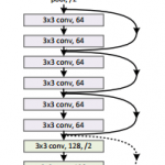
Now, before implementing the Script Module in NodeJS, let’s first trace a ResNet network using PyTorch (using just Python):
traced_net = torch.jit.trace(torchvision.models.resnet18(),
                             torch.rand(1, 3, 224, 224))
traced_net.save("resnet18_trace.pt")
As you can see from the code above, we just have to provide a tensor example (in this case a batch of a single image with 3 channels and size 224×224. After that we just save the traced network into a file called resnet18_trace.pt.
Now we’re ready to implement the Script Module in NodeJS in order to load this file that was traced.
This is now the implementation of the Script Module in NodeJS:
// Class constructor
ScriptModule::ScriptModule(const std::string filename) {
  // Load the traced network from the file
  this->mModule = torch::jit::load(filename);
}

// JavaScript object creation
NAN_METHOD(ScriptModule::New) {
  if (info.IsConstructCall()) {
    // Get the filename parameter
    v8::String::Utf8Value param_filename(info[0]->ToString());
    const std::string filename = std::string(*param_filename);

    // Create a new script module using that file name
    ScriptModule *obj = new ScriptModule(filename);
    obj->Wrap(info.This());
    info.GetReturnValue().Set(info.This());
  } else {
    v8::Local<v8::Function> cons = Nan::New(constructor);
    info.GetReturnValue().Set(Nan::NewInstance(cons).ToLocalChecked());
  }
}
As you can see from the code above, we’re just creating a class that will call the torch::jit::load function passing a file name of the traced network. We also have the implementation of the JavaScript object, where we convert parameters to C++ types and then create a new instance of the torchjs::ScriptModule.
The wrapping of the forward pass is also quite straightforward:
NAN_METHOD(ScriptModule::forward) {
  ScriptModule* script_module = ObjectWrap::Unwrap<ScriptModule>(info.Holder());
  Nan::MaybeLocal<v8::Object> maybe = Nan::To<v8::Object>(info[0]);

  Tensor *tensor =
    Nan::ObjectWrap::Unwrap<Tensor>(maybe.ToLocalChecked());

  torch::Tensor torch_tensor = tensor->getTensor();
  torch::Tensor output = script_module->mModule->forward({torch_tensor}).toTensor();

  auto newinst = Tensor::NewInstance();
  Tensor* obj = Nan::ObjectWrap::Unwrap<Tensor>(newinst);
  obj->setTensor(output);
  info.GetReturnValue().Set(newinst);
}
As you can see, in this code, we just receive a tensor as an argument, we get the internal torch::Tensor from it and then call the forward method from the script module, we wrap the output on a new torchjs::Tensor and then return it.
And that’s it, we’re ready to use our built module in native NodeJS as in the example below:
var torchjs = require("./build/Release/torchjs");
var script_module = new torchjs.ScriptModule("resnet18_trace.pt");
var data = torchjs.ones([1, 3, 224, 224], false);
var output = script_module.forward(data);
I hope you enjoyed ! Libtorch opens the door for the tight integration of PyTorch in many different languages and frameworks, which is quite exciting and a huge step towards the direction of production deployment code.
– Christian S. Perone
Concentration inequalities, or probability bounds, are very important tools for the analysis of Machine Learning algorithms or randomized algorithms. In statistical learning theory, we often want to show that random variables, given some assumptions, are close to its expectation with high probability. This article provides an overview of the most basic inequalities in the analysis of these concentration measures.
The Markov’s inequality is one of the most basic bounds and it assumes almost nothing about the random variable. The assumptions that Markov’s inequality makes is that the random variable \(X\) is non-negative \(X > 0\) and has a finite expectation \(\mathbb{E}\left[X\right] < \infty\). The Markov’s inequality is given by:
$$\underbrace{P(X \geq \alpha)}_{\text{Probability of being greater than constant } \alpha} \leq \underbrace{\frac{\mathbb{E}\left[X\right]}{\alpha}}_{\text{Bounded above by expectation over constant } \alpha}$$
What this means is that the probability that the random variable \(X\) will be bounded by the expectation of \(X\) divided by the constant \(\alpha\). What is remarkable about this bound, is that it holds for any distribution with positive values and it doesn’t depend on any feature of the probability distribution, it only requires some weak assumptions and its first moment, the expectation.
Example: A grocery store sells an average of 40 beers per day (it’s summer !). What is the probability that it will sell 80 or more beers tomorrow ?
$$
\begin{align}
P(X \geq \alpha) & \leq\frac{\mathbb{E}\left[X\right]}{\alpha} \\\\
P(X \geq 80) & \leq\frac{40}{80} = 0.5 = 50\%
\end{align}
$$
The Markov’s inequality doesn’t depend on any property of the random variable probability distribution, so it’s obvious that there are better bounds to use if information about the probability distribution is available.
When we have information about the underlying distribution of a random variable, we can take advantage of properties of this distribution to know more about the concentration of this variable. Let’s take for example a normal distribution with mean \(\mu = 0\) and unit standard deviation \(\sigma = 1\) given by the probability density function (PDF) below:
$$ f(x) = \frac{1}{\sqrt{2\pi}}e^{-x^2/2} $$
Integrating from -1 to 1: \(\int_{-1}^{1} \frac{1}{\sqrt{2\pi}}e^{-x^2/2}\), we know that 68% of the data is within \(1\sigma\) (one standard deviation) from the mean \(\mu\) and 95% is within \(2\sigma\) from the mean. However, when it’s not possible to assume normality, any other amount of data can be concentrated within \(1\sigma\) or \(2\sigma\).
Chebyshev’s inequality provides a way to get a bound on the concentration for any distribution, without assuming any underlying property except a finite mean and variance. Chebyshev’s also holds for any random variable, not only for non-negative variables as in Markov’s inequality.
The Chebyshev’s inequality is given by the following relation:
$$
P( \mid X – \mu \mid \geq k\sigma) \leq \frac{1}{k^2}
$$
that can also be rewritten as:
$$
P(\mid X – \mu \mid < k\sigma) \geq 1 – \frac{1}{k^2}
$$
For the concrete case of \(k = 2\), the Chebyshev’s tells us that at least 75% of the data is concentrated within 2 standard deviations of the mean. And this holds for any distribution.
Now, when we compare this result for \( k = 2 \) with the 95% concentration of the normal distribution for \(2\sigma\), we can see how conservative is the Chebyshev’s bound. However, one must not forget that this holds for any distribution and not only for a normally distributed random variable, and all that Chebyshev’s needs, is the first and second moments of the data. Something important to note is that in absence of more information about the random variable, this cannot be improved.
Chebyshev’s inequality can also be used to prove the weak law of large numbers, which says that the sample mean converges in probability towards the true mean.
That can be done as follows:
Before getting into the Chernoff bound, let’s understand the motivation behind it and how one can improve on Chebyshev’s bound. To understand it, we first need to understand the difference between a pairwise independence and mutual independence. For the pairwise independence, we have the following for A, B, and C:
$$
P(A \cap B) = P(A)P(B) \\
P(A \cap C) = P(A)P(C) \\
P(B \cap C) = P(B)P(C)
$$
Which means that any pair (any two events) are independent, but not necessarily that:
$$
P(A \cap B\cap C) = P(A)P(B)P(C)
$$
which is called “mutual independence” and it is a stronger independence. By definition, the mutual independence assumes the pairwise independence but the opposite isn’t always true. And this is the case where we can improve on Chebyshev’s bound, as it is not possible without doing these further assumptions (stronger assumptions leads to stronger bounds).
We’ll talk about the Chernoff bounds in the second part of this tutorial !