Tag: uncertainty

Machine Learning

Couple of recent publications in uncertainty estimation and autonomous vehicles

Just sharing some recent publications I’ve been involved recently:

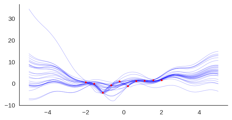
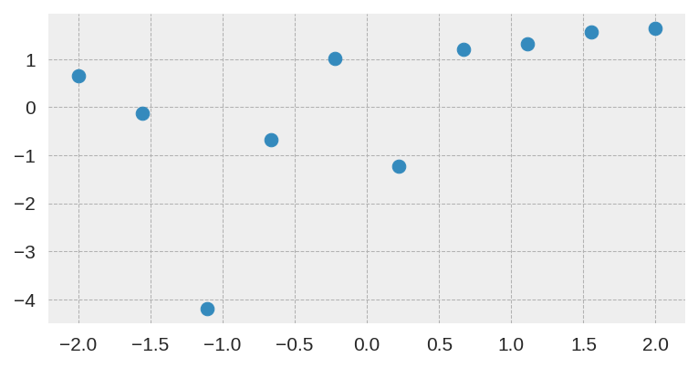
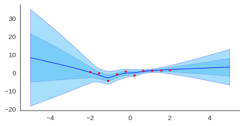
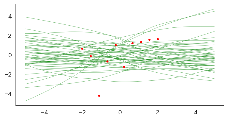
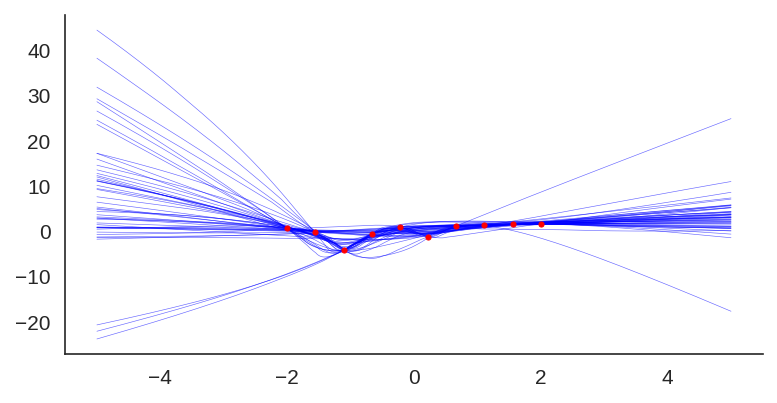
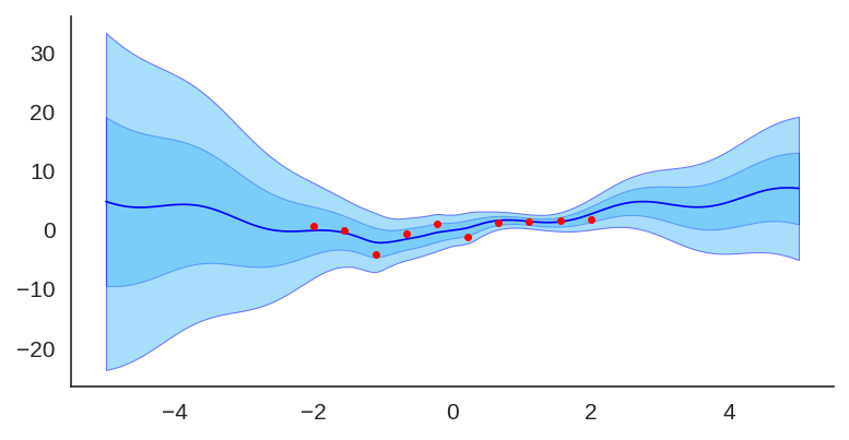
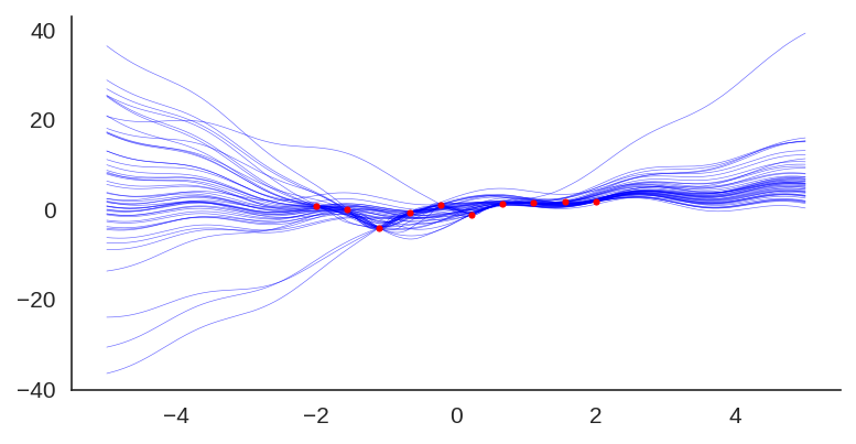
L2M: Practical posterior Laplace approximation with optimization-driven second moment estimation

ArXiv: https://arxiv.org/abs/2107.04695 (ICML 2021 / UDL)

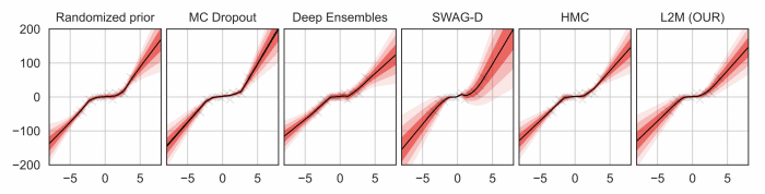
Uncertainty quantification for deep neural networks has recently evolved through many techniques. In this work, we revisit Laplace approximation, a classical approach for posterior approximation that is computationally attractive. However, instead of computing the curvature matrix, we show that, under some regularity conditions, the Laplace approximation can be easily constructed using the gradient second moment. This quantity is already estimated by many exponential moving average variants of Adagrad such as Adam and RMSprop, but is traditionally discarded after training. We show that our method (L2M) does not require changes in models or optimization, can be implemented in a few lines of code to yield reasonable results, and it does not require any extra computational steps besides what is already being computed by optimizers, without introducing any new hyperparameter. We hope our method can open new research directions on using quantities already computed by optimizers for uncertainty estimation in deep neural networks.

CW-ERM: Improving Autonomous Driving Planning with Closed-loop Weighted Empirical Risk Minimization

ArXiv: https://arxiv.org/abs/2210.02174 (NeurIPS 2022 / ML4AD / ICRA 2023 under review)

Project page: https://woven.mobi/cw-erm

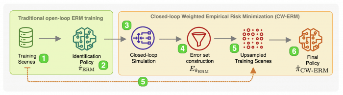
The imitation learning of self-driving vehicle policies through behavioral cloning is often carried out in an open-loop fashion, ignoring the effect of actions to future states. Training such policies purely with Empirical Risk Minimization (ERM) can be detrimental to real-world performance, as it biases policy networks towards matching only open-loop behavior, showing poor results when evaluated in closed-loop. In this work, we develop an efficient and simple-to-implement principle called Closed-loop Weighted Empirical Risk Minimization (CW-ERM), in which a closed-loop evaluation procedure is first used to identify training data samples that are important for practical driving performance and then we these samples to help debias the policy network. We evaluate CW-ERM in a challenging urban driving dataset and show that this procedure yields a significant reduction in collisions as well as other non-differentiable closed-loop metrics.

SafePathNet: Safe Real-World Autonomous Driving by Learning to Predict and Plan with a Mixture of Experts

ArXiv: https://arxiv.org/abs/2211.02131 (NeurIPS 2022 / ML4AD / ICRA 2023 under review)

Project page: https://woven.mobi/safepathnet

The goal of autonomous vehicles is to navigate public roads safely and comfortably. To enforce safety, traditional planning approaches rely on handcrafted rules to generate trajectories. Machine learning-based systems, on the other hand, scale with data and are able to learn more complex behaviors. However, they often ignore that agents and self-driving vehicle trajectory distributions can be leveraged to improve safety. In this paper, we propose modeling a distribution over multiple future trajectories for both the self-driving vehicle and other road agents, using a unified neural network architecture for prediction and planning. During inference, we select the planning trajectory that minimizes a cost taking into account safety and the predicted probabilities. Our approach does not depend on any rule-based planners for trajectory generation or optimization, improves with more training data and is simple to implement. We extensively evaluate our method through a realistic simulator and show that the predicted trajectory distribution corresponds to different driving profiles. We also successfully deploy it on a self-driving vehicle on urban public roads, confirming that it drives safely without compromising comfort.

Machine Learning

Uncertainty Estimation in Deep Learning (PyData Lisbon / July 2019)

Just sharing some slides I presented at the PyData Lisbon on July 2019 about the talk “Uncertainty Estimation in Deep Learning“:

Cite this article as: Christian S. Perone, "Uncertainty Estimation in Deep Learning (PyData Lisbon / July 2019)," in Terra Incognita, 18/07/2019, https://blog.christianperone.com/2019/07/uncertainty-estimation-in-deep-learning-pydata-lisbon-july-2019/.
Machine Learning, Python

Randomized prior functions in PyTorch

Trained MLP with 2 hidden layers and a sine prior.

I was experimenting with the approach described in “Randomized Prior Functions for Deep Reinforcement Learning” by Ian Osband et al. at NPS 2018, where they devised a very simple and practical method for uncertainty using bootstrap and randomized priors and decided to share the PyTorch code.

I really like bootstrap approaches, and in my opinion, they are usually the easiest methods to implement and provide very good posterior approximation with deep connections to Bayesian approaches, without having to deal with variational inference. They actually show in the paper that in the linear case, the method provides a Bayes posterior.

The main idea of the method is to have bootstrap to provide a non-parametric data perturbation together with randomized priors, which are nothing more than just random initialized networks.

$$Q_{\theta_k}(x) = f_{\theta_k}(x) + p_k(x)$$

The final model \(Q_{\theta_k}(x)\) will be the k model of the ensemble that will fit the function \(f_{\theta_k}(x)\) with an untrained prior \(p_k(x)\).

Let’s go to the code. The first class is a simple MLP with 2 hidden layers and Glorot initialization :

class MLP(nn.Module):
    def __init__(self):
        super().__init__()
        self.l1 = nn.Linear(1, 20)
        self.l2 = nn.Linear(20, 20)
        self.l3 = nn.Linear(20, 1)
        
        nn.init.xavier_uniform_(self.l1.weight)
        nn.init.xavier_uniform_(self.l2.weight)
        nn.init.xavier_uniform_(self.l3.weight)

    def forward(self, inputs):
        x = self.l1(inputs)
        x = nn.functional.selu(x)
        x = self.l2(x)
        x = nn.functional.selu(x)
        x = self.l3(x)
        return x

Then later we define a class that will take the model and the prior to produce the final model result:

class ModelWithPrior(nn.Module):
    def __init__(self,
                 base_model : nn.Module,
                 prior_model : nn.Module,
                 prior_scale : float = 1.0):
        super().__init__()
        self.base_model = base_model
        self.prior_model = prior_model
        self.prior_scale = prior_scale

    def forward(self, inputs):
        with torch.no_grad():
            prior_out = self.prior_model(inputs)
            prior_out = prior_out.detach()
        model_out = self.base_model(inputs)
        return model_out + (self.prior_scale * prior_out)

And it’s basically that ! As you can see, it’s a very simple method, in the second part we just created a custom forward() to avoid computing/accumulating gradients for the prior network and them summing (after scaling) it with the model prediction.

To train it, you just have to use different bootstraps for each ensemble model, like in the code below:

def train_model(x_train, y_train, base_model, prior_model):
    model = ModelWithPrior(base_model, prior_model, 1.0)
    loss_fn = nn.MSELoss()
    optimizer = torch.optim.Adam(model.parameters(), lr=0.05)
    
    for epoch in range(100):
        model.train()
        preds = model(x_train)
        loss = loss_fn(preds, y_train)

        optimizer.zero_grad()
        loss.backward()
        optimizer.step()
            
    return model

and using a sampler with replacement (bootstrap) as in:

dataset = TensorDataset(...)
bootstrap_sampler = RandomSampler(dataset, True, len(dataset))
train_dataloader = DataLoader(dataset,
                              batch_size=len(dataset),
                              sampler=bootstrap_sampler)

In this case, I used the same small dataset used in the original paper:

After training it with a simple MLP prior as well, the results for the uncertainty are shown below:

Trained model with an MLP prior, used an ensemble of 50 models.

If we look at just the priors, we will see the variation of the untrained networks:

We can also visualize the individual model predictions showing their variability due to different initializations as well as the bootstrap noise:

Plot showing each individual model prediction and true data in red.

Now, what is also quite interesting, is that we can change the prior to let’s say a fixed sine:

class SinPrior(nn.Module):
    def forward(self, input):
        return torch.sin(3 * input)

Then, when we train the same MLP model but this time using the sine prior, we can see how it affects the final prediction and uncertainty bounds:

If we show each individual model, we can see the effect of the prior contribution to each individual model:

Plot showing each individual model of the ensemble trained with a sine prior.

I hope you liked, these are quite amazing results for a simple method that at least pass the linear “sanity check”. I’ll explore some pre-trained networks in place of the prior to see the different effects on predictions, it’s a very interesting way to add some simple priors.

Cite this article as: Christian S. Perone, "Randomized prior functions in PyTorch," in Terra Incognita, 24/03/2019, https://blog.christianperone.com/2019/03/randomized-prior-functions-in-pytorch/.

I'm starting a new course "Machine Learning: Foundations and Engineering" for 2024.