The new generation of OpenCV bindings for Python is getting better and better with the hard work of the community. The new bindings, called “cv2” are the replacement of the old “cv” bindings; in this new generation of bindings, almost all operations returns now native Python objects or Numpy objects, which is pretty nice since it simplified a lot and also improved performance on some areas due to the fact that you can now also use the optimized operations from Numpy and also enabled the integration with other frameworks like the scikit-image which also uses Numpy arrays for image representation.
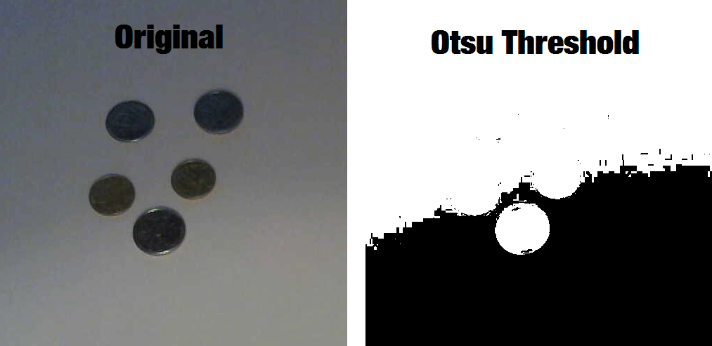
In this example, I’ll show how to segment coins present in images or even real-time video capture with a simple approach using thresholding, morphological operators, and contour approximation. This approach is a lot simpler than the approach using Otsu’s thresholding and Watershed segmentation here in OpenCV Python tutorials, which I highly recommend you to read due to its robustness. Unfortunately, the approach using Otsu’s thresholding is highly dependent on an illumination normalization. One could extract small patches of the image to implement something similar to an adaptive Otsu’s binarization (like the one implemented in Letptonica – the framework used by Tesseract OCR) to overcome this problem, but let’s see another approach. For reference, see the output of the Otsu’s thresholding using an image taken with my webcam with a non-normalized illumination:
1. Setting the Video Capture configuration
The first step to create a real-time Video Capture using the Python bindings is to instantiate the VideoCapture class, set the properties and then start reading frames from the camera:
import numpy as np
import cv2

cap = cv2.VideoCapture(0)
cap.set(cv2.cv.CV_CAP_PROP_FRAME_WIDTH, 1280)
cap.set(cv2.cv.CV_CAP_PROP_FRAME_HEIGHT, 720)
In newer versions (unreleased yet), the constants for CV_CAP_PROP_FRAME_WIDTH are now in the cv2 module, for now, let’s just use the cv2.cv module.
2. Reading image frames
The next step is to use the VideoCapture object to read the frames and then convert them to gray color (we are not going to use color information to segment the coins):
while True:
    ret, frame = cap.read()
    roi = frame[0:500, 0:500]
    gray = cv2.cvtColor(roi, cv2.COLOR_BGR2GRAY)
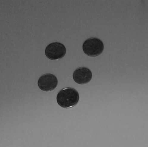
Note that here I’m extracting a small portion of the complete image (where the coins are located), but you don’t have to do that if you have only coins on your image. At this moment, we have the following gray image:
3. Applying adaptive thresholding
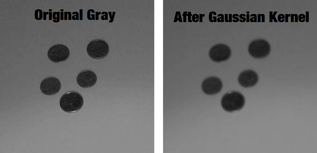
In this step we will apply the Adaptive Thresholding after applying a Gaussian Blur kernel to eliminate the noise that we have in the image:
gray_blur = cv2.GaussianBlur(gray, (15, 15), 0)
thresh = cv2.adaptiveThreshold(gray_blur, 255, cv2.ADAPTIVE_THRESH_GAUSSIAN_C,
cv2.THRESH_BINARY_INV, 11, 1)
See the effect of the Gaussian Kernel in the image:
And now the effect of the Adaptive Thresholding with the blurry image:
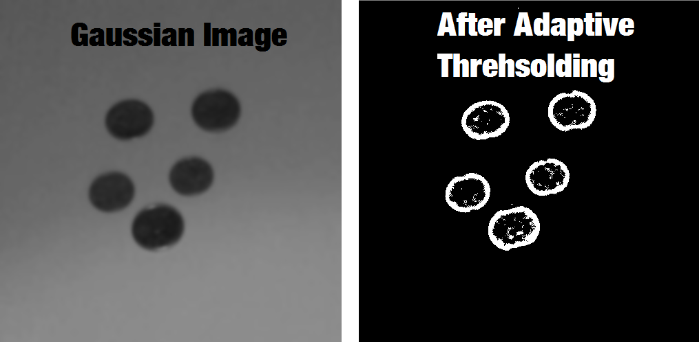
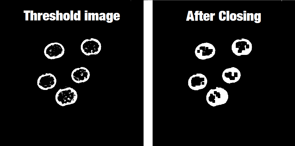
Note that at that moment we already have the coins segmented except for the small noisy inside the center of the coins and also in some places around them.
4. Morphology
The Morphological Operators are used to dilate, erode and other operations on the pixels of the image. Here, due to the fact that sometimes the camera can present some artifacts, we will use the Morphological Operation of Closing to make sure that the borders of the coins are always close, otherwise, we may found a coin with a semi-circle or something like that. To understand the effect of the Closing operation (which is the operation of erosion of the pixels already dilated) see the image below:
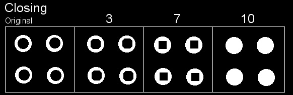
You can see that after some iterations of the operation, the circles start to become filled. To use the Closing operation, we’ll use the morphologyEx function from the OpenCV Python bindings:
kernel = np.ones((3, 3), np.uint8)
closing = cv2.morphologyEx(thresh, cv2.MORPH_CLOSE, kernel, iterations=4)
See now the effect of the Closing operation on our coins:
The operations of Morphological Operators are very simple, the main principle is the application of an element (in our case we have a block element of 3×3) into the pixels of the image. If you want to understand it, please see this animation explaining the operation of Erosion.
5. Contour detection and filtering
After applying the morphological operators, all we have to do is to find the contour of each coin and then filter the contours having an area smaller or larger than a coin area. You can imagine the procedure of finding contours in OpenCV as the operation of finding connected components and their boundaries. To do that, we’ll use the OpenCV findContours function.
cont_img = closing.copy()
contours, hierarchy = cv2.findContours(cont_img, cv2.RETR_EXTERNAL,
cv2.CHAIN_APPROX_SIMPLE)
Note that we made a copy of the closing image because the function findContours will change the image passed as the first parameter, we’re also using the RETR_EXTERNAL flag, which means that the contours returned are only the extreme outer contours. The parameter CHAIN_APPROX_SIMPLE will also return a compact representation of the contour, for more information see here.
After finding the contours, we need to iterate into each one and check the area of them to filter the contours containing an area greater or smaller than the area of a coin. We also need to fit an ellipse to the contour found. We could have done this using the minimum enclosing circle, but since my camera isn’t perfectly above the coins, the coins appear with a small inclination describing an ellipse.
for cnt in contours:
area = cv2.contourArea(cnt)
if area < 2000 or area > 4000:
continue
if len(cnt) < 5:
continue
ellipse = cv2.fitEllipse(cnt)
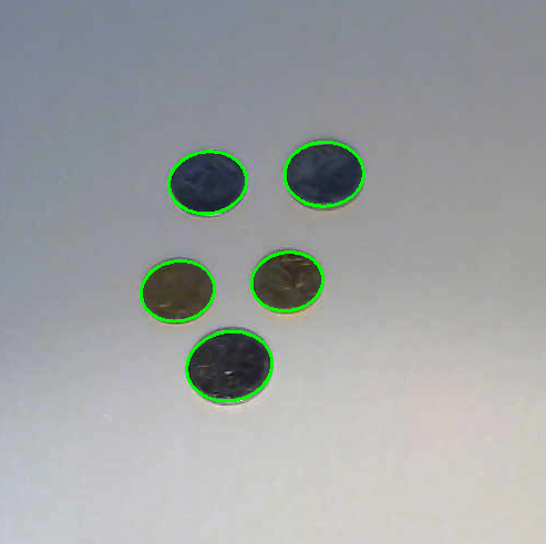
cv2.ellipse(roi, ellipse, (0,255,0), 2)
Note that in the code above we are iterating on each contour, filtering coins with area smaller than 2000 or greater than 4000 (these are hardcoded values I found for the Brazilian coins at this distance from the camera), later we check for the number of points of the contour because the function fitEllipse needs a number of points greater or equal than 5 and finally we use the ellipse function to draw the ellipse in green over the original image.
To show the final image with the contours we just use the imshow function to show a new window with the image:
cv2.imshow('final result', roi)
And finally, this is the result in the end of all steps described above:
The complete source-code:
import numpy as np
import cv2

def run_main():
    cap = cv2.VideoCapture(0)
    cap.set(cv2.cv.CV_CAP_PROP_FRAME_WIDTH, 1280)
    cap.set(cv2.cv.CV_CAP_PROP_FRAME_HEIGHT, 720)

    while(True):
        ret, frame = cap.read()
        roi = frame[0:500, 0:500]
        gray = cv2.cvtColor(roi, cv2.COLOR_BGR2GRAY)

        gray_blur = cv2.GaussianBlur(gray, (15, 15), 0)
        thresh = cv2.adaptiveThreshold(gray_blur, 255, cv2.ADAPTIVE_THRESH_GAUSSIAN_C,
                                       cv2.THRESH_BINARY_INV, 11, 1)

        kernel = np.ones((3, 3), np.uint8)
        closing = cv2.morphologyEx(thresh, cv2.MORPH_CLOSE,
        kernel, iterations=4)

        cont_img = closing.copy()
        contours, hierarchy = cv2.findContours(cont_img, cv2.RETR_EXTERNAL,
                                               cv2.CHAIN_APPROX_SIMPLE)

        for cnt in contours:
            area = cv2.contourArea(cnt)
            if area < 2000 or area > 4000:
                continue

            if len(cnt) < 5:
                continue

            ellipse = cv2.fitEllipse(cnt)
            cv2.ellipse(roi, ellipse, (0,255,0), 2)

        cv2.imshow("Morphological Closing", closing)
        cv2.imshow("Adaptive Thresholding", thresh)
        cv2.imshow('Contours', roi)

        if cv2.waitKey(1) & 0xFF == ord('q'):
            break

    cap.release()
    cv2.destroyAllWindows()

if __name__ == "__main__":
    run_main()
") and
and ") , where
, where  and
and  are the components of the vector (features of the document, or TF-IDF values for each word of the document in our example) and the
  is the dimension of the vectors:
 \\ \vec{b} = (4, 0) \\ \vec{a} \cdot \vec{b} = 0*4 + 3*0 = 0")


 ? This term is the projection of the vector
  into the vector
  as shown on the image below:

 :
:


 ) and move the
  to the right hand of the equation:
 is the same as the inverse of the cosine (
 ).
).


